2. R Code
# Update Packages
update.packages(ask = FALSE, repos='https://cran.csiro.au/', dependencies = TRUE)
# preparation
if (!require("sjlabelled")) install.packages("sjlabelled", dependencies = TRUE)
if (!require("sjmisc")) install.packages("sjmisc", dependencies = TRUE)
if (!require("sjPlot")) install.packages("sjPlot", dependencies = TRUE)
if (!require("dplyr")) install.packages("dplyr", dependencies = TRUE)
if (!require("ggrepel")) install.packages("ggrepel", dependencies = TRUE)
if (!require("Hmisc")) install.packages("Hmisc", dependencies = TRUE)
if (!require("ggplot2")) install.packages("ggplot2", dependencies = TRUE)
if (!require("ggthemes")) install.packages("ggthemes", dependencies = TRUE)
library(sjlabelled)
library(sjmisc)
library(sjPlot)
library(dplyr)
library(ggrepel)
library(Hmisc)
library(ggplot2)
library(ggthemes)

# data
aus2012 <- readRDS(url("https://mqsociology.github.io/learn-r/soci832/aussa2012.RDS"))
lga <- readRDS(url("https://mqsociology.github.io/learn-r/soci832/nsw-lga-crime.RDS"))

# Turn off scientific notation
options(digits=3, scipen=8)

# Stop View from overloading memory with a large datasets
RStudioView <- View
View <- function(x) {
  if ("data.frame" %in% class(x)) { RStudioView(x[1:500,]) } else { RStudioView(x) }
}
my_theme <-   theme_classic(base_size = 12)  +
  theme(
    plot.title = element_text(hjust = 0.5, size = 14, color="red", face="bold.italic"),    # Center title position and size
    plot.subtitle = element_text(hjust = 0.5),            # Center subtitle
    plot.caption = element_text(hjust = 0, face = "italic"), # move caption to the left
    axis.title.x = element_text(color="blue", size=14, face="bold"),
    axis.title.y = element_text(color="#993333", size=14, face="bold")
  )

################################################################################
# 1. Bar graph
################################################################################
# 1.1 Basic bar graph
plot_frq(aus2012$fechld, type = "bar")  + my_theme
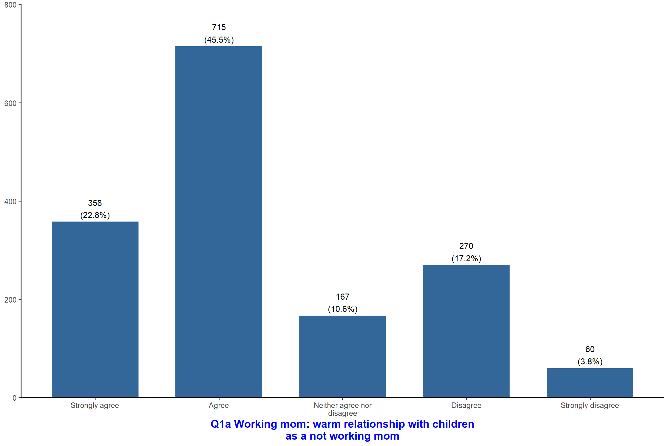
plot_frq(aus2012$fechld, type = "bar", title = "Attitude toward working mom") + my_theme # Add the title

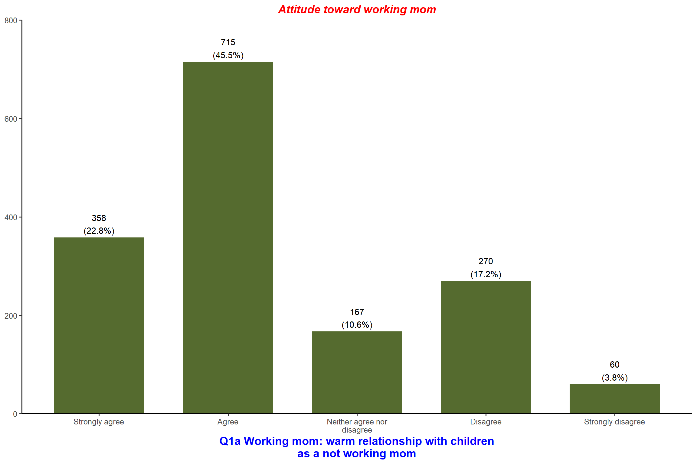
plot_frq(aus2012$fechld, type = "bar", title = "Attitude toward working mom",
        geom.colors = "darkolivegreen")  + my_theme  # Change bar color
plot_frq(aus2012$fechld, type = "bar", title = "Attitude toward working mom",
        show.values = FALSE)   + my_theme  # do not show values

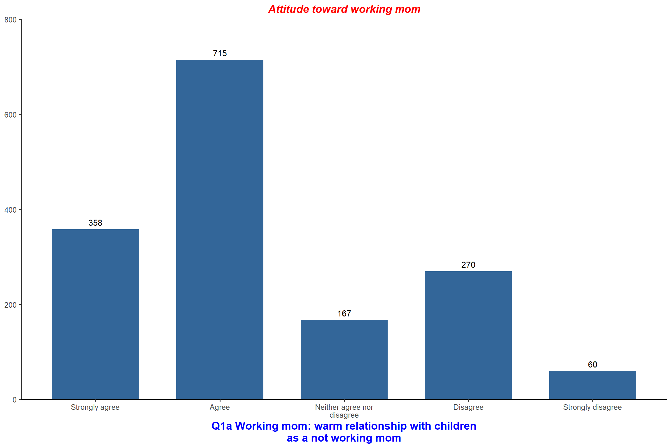
plot_frq(aus2012$fechld, type = "bar", title = "Attitude toward working mom",
        show.prc = FALSE)  + my_theme  # do not show percentages
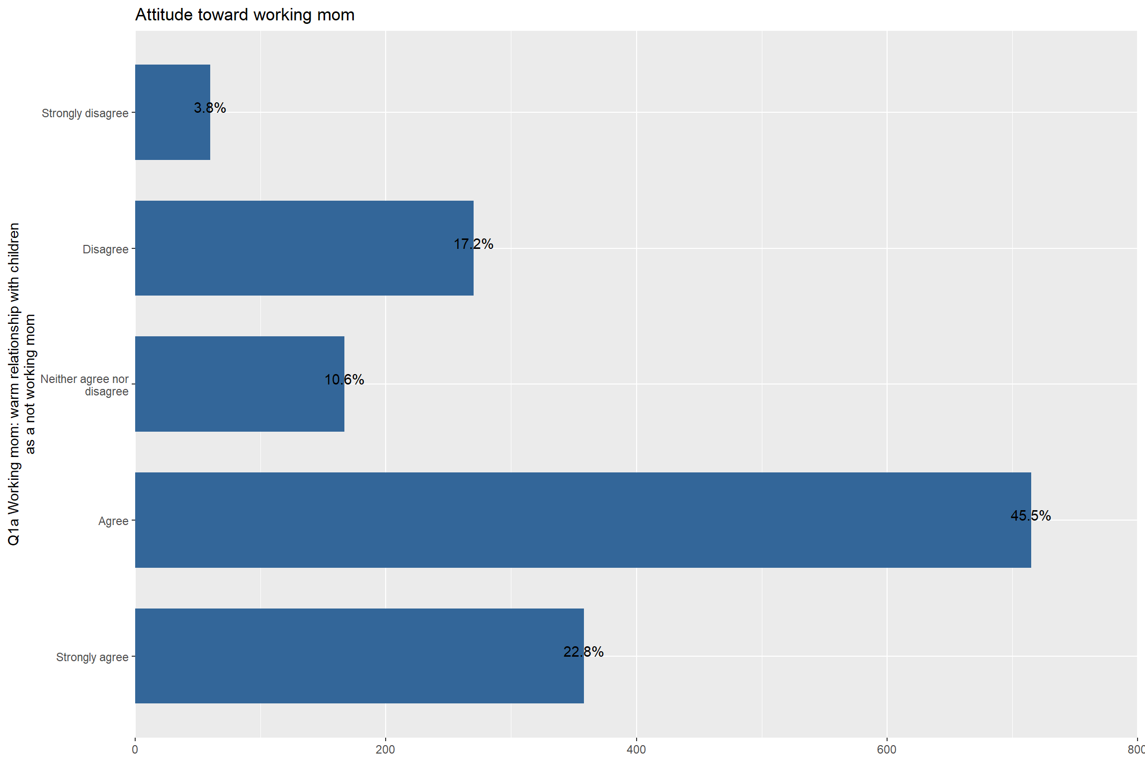
plot_frq(aus2012$fechld,
        type = "bar",
        title = "Attitude toward working mom",
        show.n = FALSE,
        coord.flip = TRUE) # do not show frequencies
# 1.2 Stacked bar graph
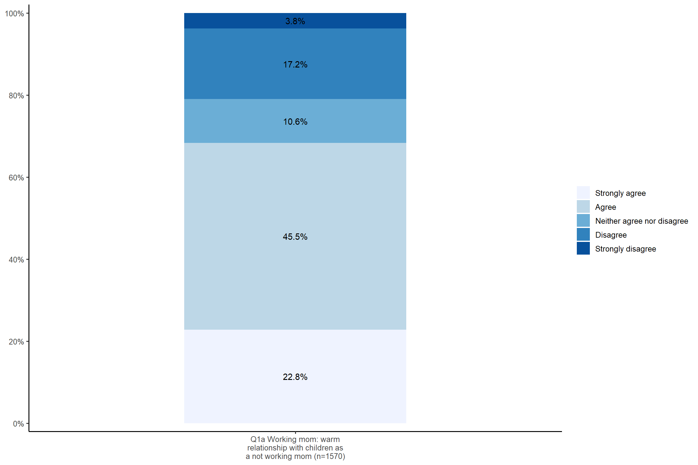
plot_stackfrq(aus2012$fechld) + my_theme
plot_stackfrq(aus2012$fechld, coord.flip = FALSE) + my_theme # the x and y axis are swaped
plot_stackfrq(aus2012[, c("fechld", "fepresch", "famsuffr", "homekid", "housewrk")]) + my_theme # plot many variables simultaneously
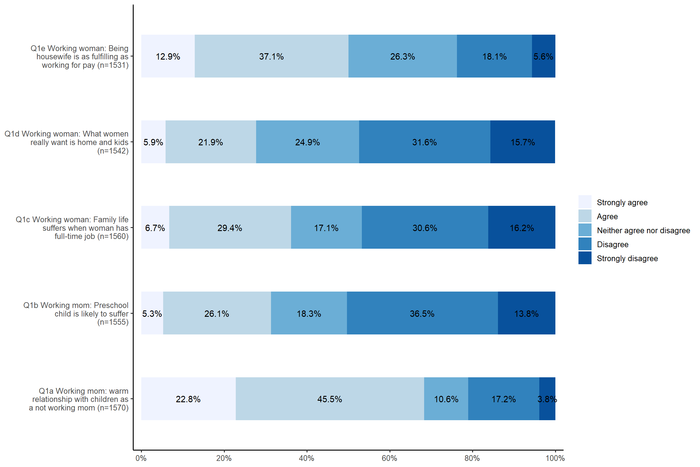
plot_stackfrq(aus2012[, c("fechld", "fepresch", "famsuffr", "homekid", "housewrk")],
             title = "Attitude toward working women (or mom)") + theme_classic()# Add the title
# 1.3 Stacked bar graph for likert scale
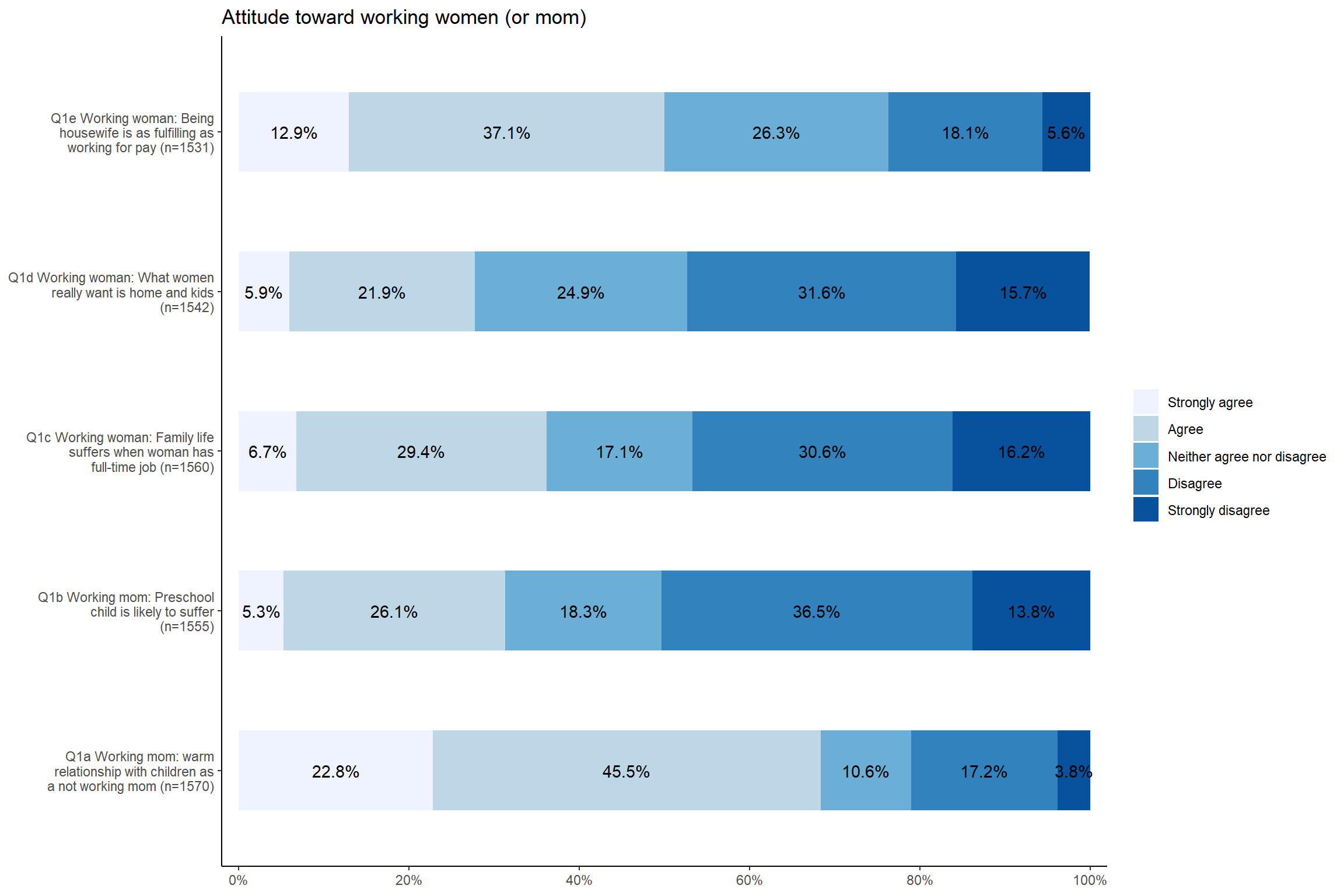
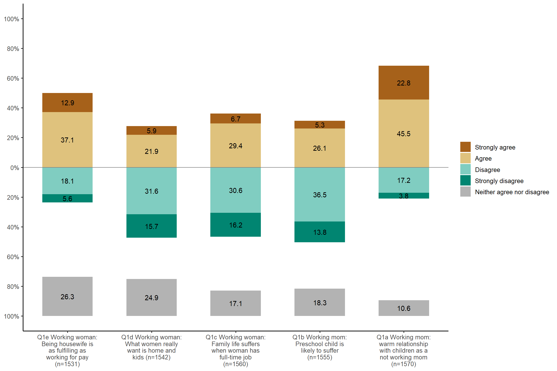
plot_likert(aus2012[, c("fechld", "fepresch", "famsuffr", "homekid", "housewrk")],
cat.neutral = 3) + my_theme # 'cat.neutral' means a neutral category such as "neither agree nor disagree".
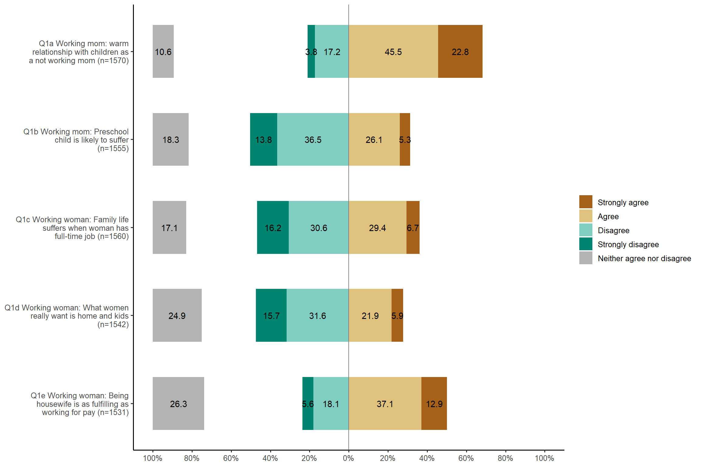
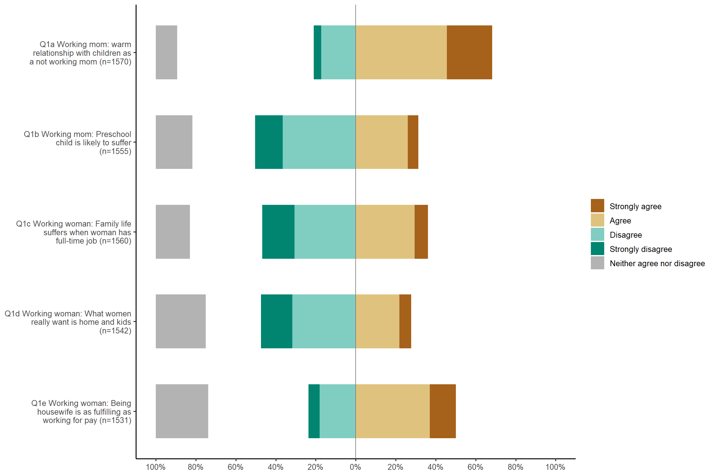
plot_likert(aus2012[, c("fechld", "fepresch", "famsuffr", "homekid", "housewrk")],
           cat.neutral = 3, values = "hide") + my_theme # hide the percentage values on the bars.
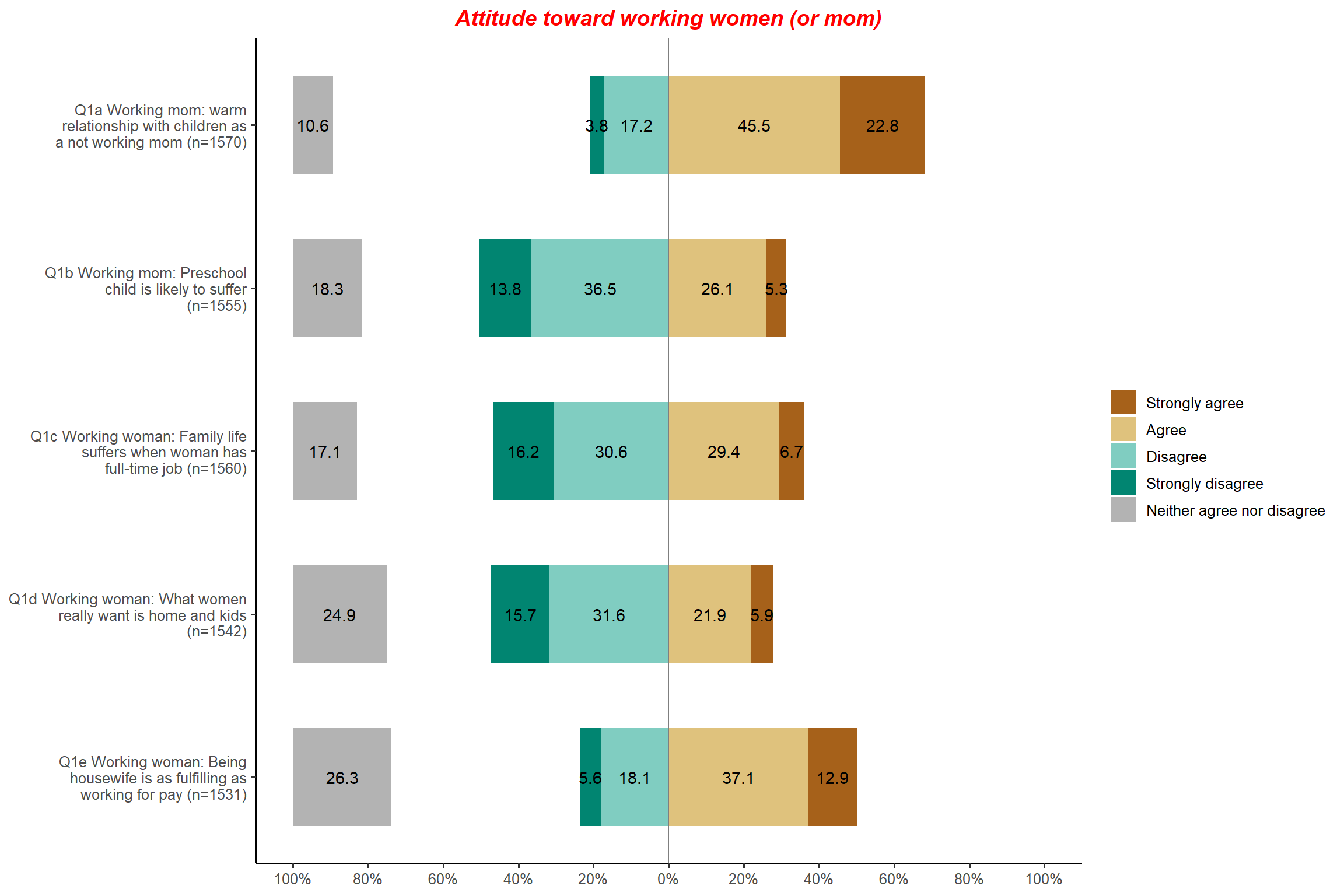
plot_likert(aus2012[, c("fechld", "fepresch", "famsuffr", "homekid", "housewrk")],
           cat.neutral = 3, title = "Attitude toward working women (or mom)") + my_theme  # Add the title
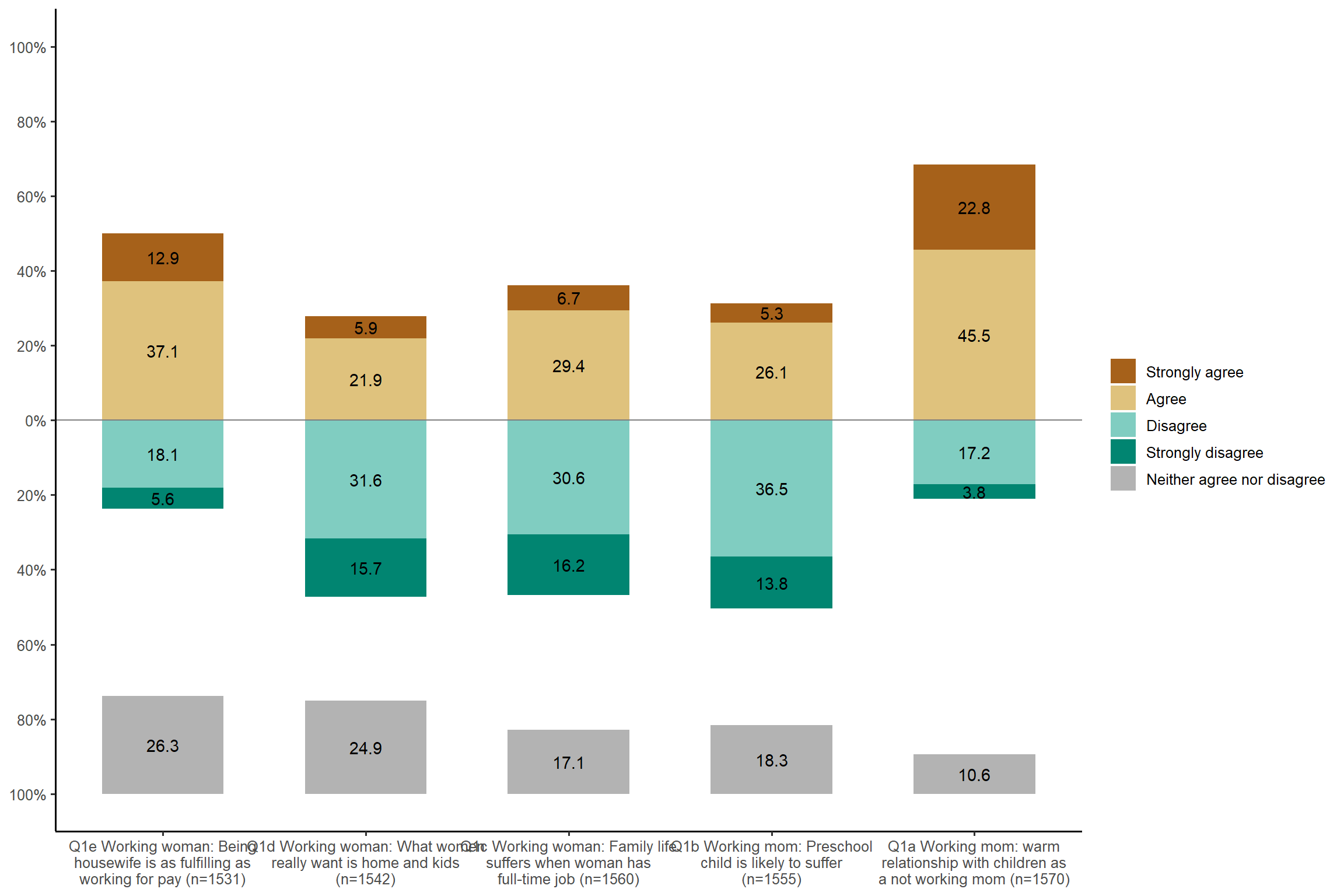
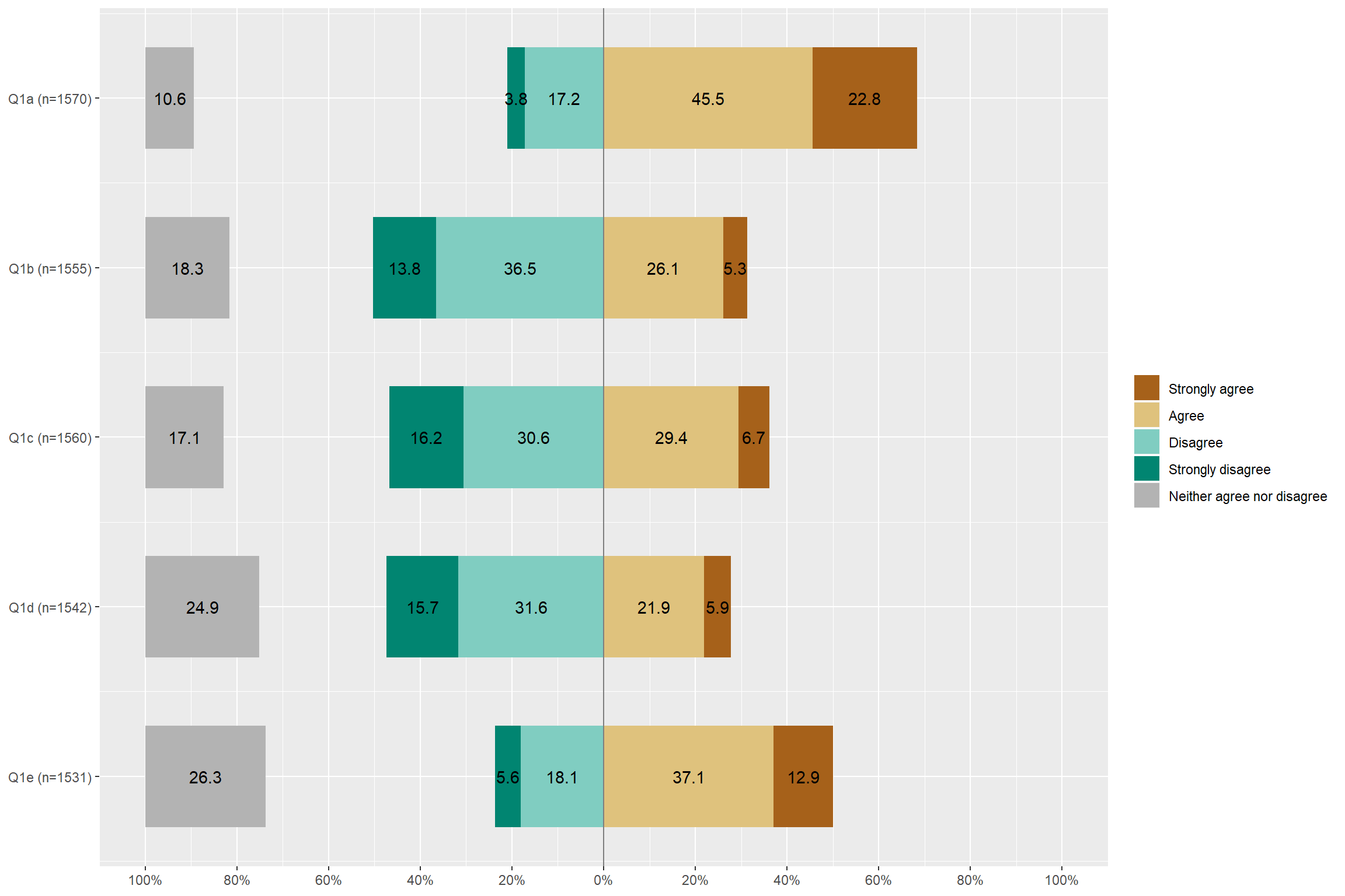
plot_likert(aus2012[, c("fechld", "fepresch", "famsuffr", "homekid", "housewrk")],
           cat.neutral = 3, coord.flip = FALSE) + my_theme # the x and y axis are swaped; but you will see the variable name is so long; I will fix them in the next code.
plot_likert(aus2012[, c("fechld", "fepresch", "famsuffr", "homekid", "housewrk")],
           cat.neutral = 3, coord.flip = FALSE, wrap.labels = 20) + my_theme # 'wrap.labels' determines how many characters are displayed in one line and when a line brek is inserted
## Also, I would like to tell you how to change variable names
wrkwm <- aus2012[, c("fechld", "fepresch", "famsuffr", "homekid", "housewrk")] # extract five variables
wrkwm$fechld <- set_label(wrkwm$fechld, label = "Q1a") # change the variable name
wrkwm$fepresch <- set_label(wrkwm$fepresch, label = "Q1b")
wrkwm$famsuffr <- set_label(wrkwm$famsuffr, label = "Q1c")
wrkwm$homekid <- set_label(wrkwm$homekid, label = "Q1d")
wrkwm$housewrk <- set_label(wrkwm$housewrk, label = "Q1e")

plot_likert(wrkwm, cat.neutral = 3)
## Note: if you want to change value labels, use 'set_labels()'.

# 1.4 Grouped bar plot
plot_xtab(aus2012$fechld, aus2012$sex)  + my_theme
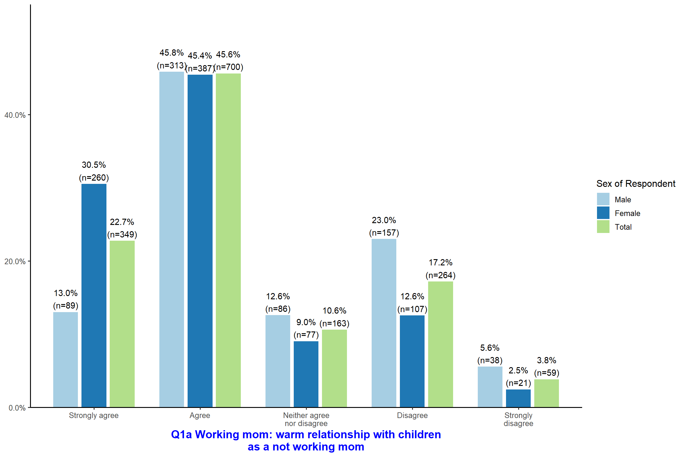
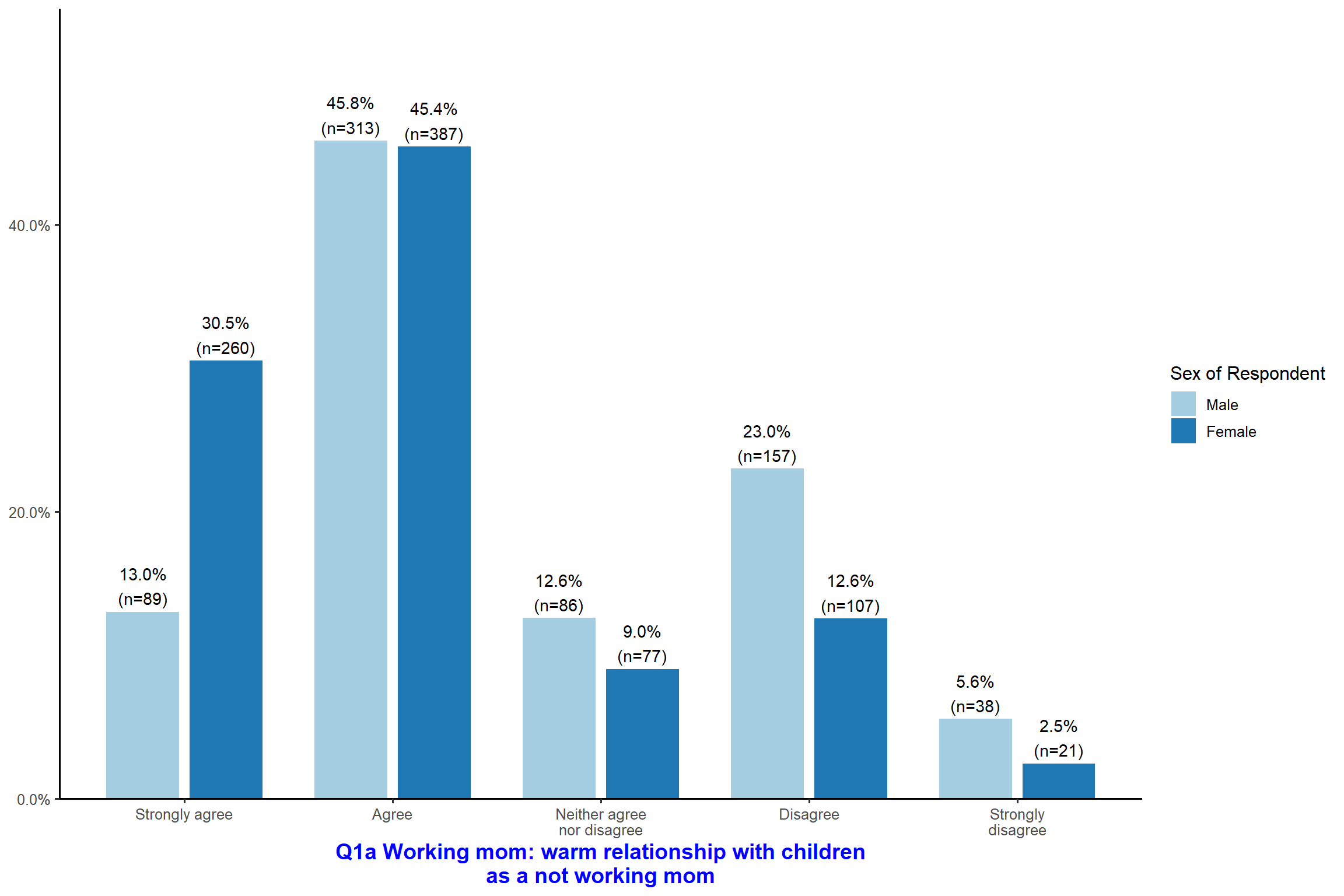
plot_xtab(aus2012$fechld, aus2012$sex, show.total = FALSE) + my_theme # do not show the total.
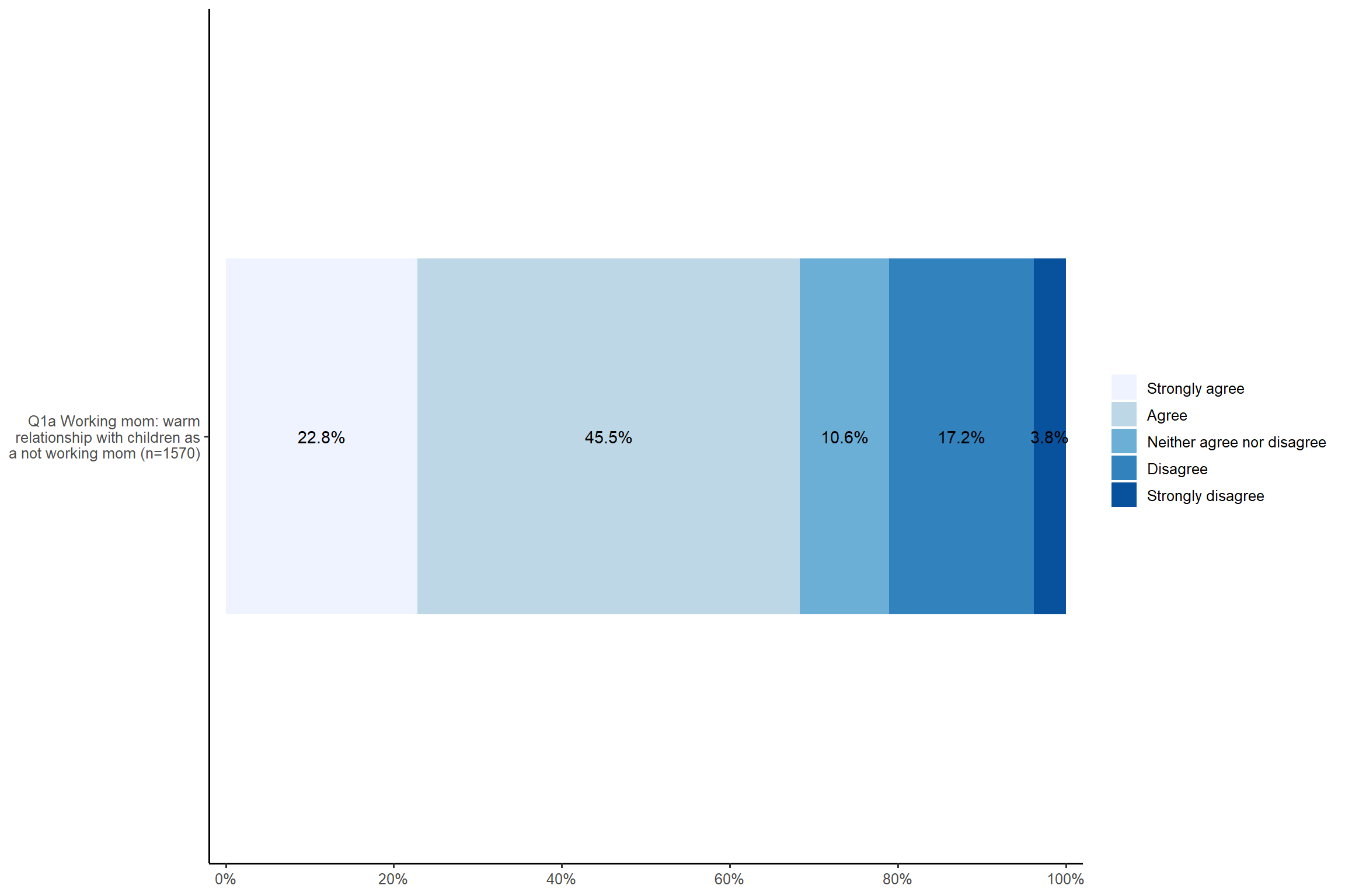
plot_xtab(aus2012$sex, aus2012$fechld, bar.pos = "stack", show.total = FALSE) + my_theme
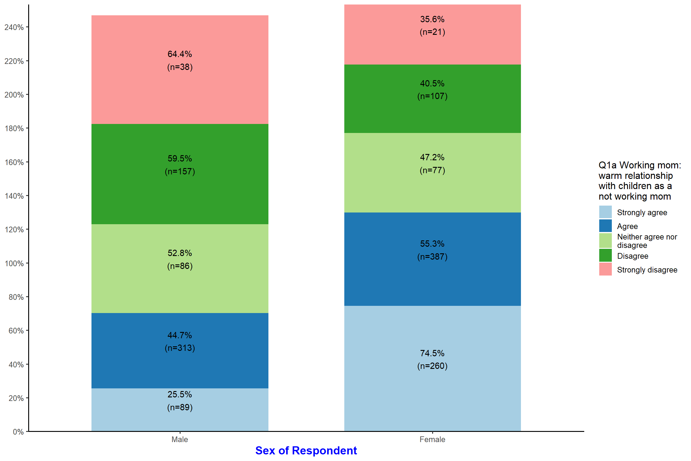
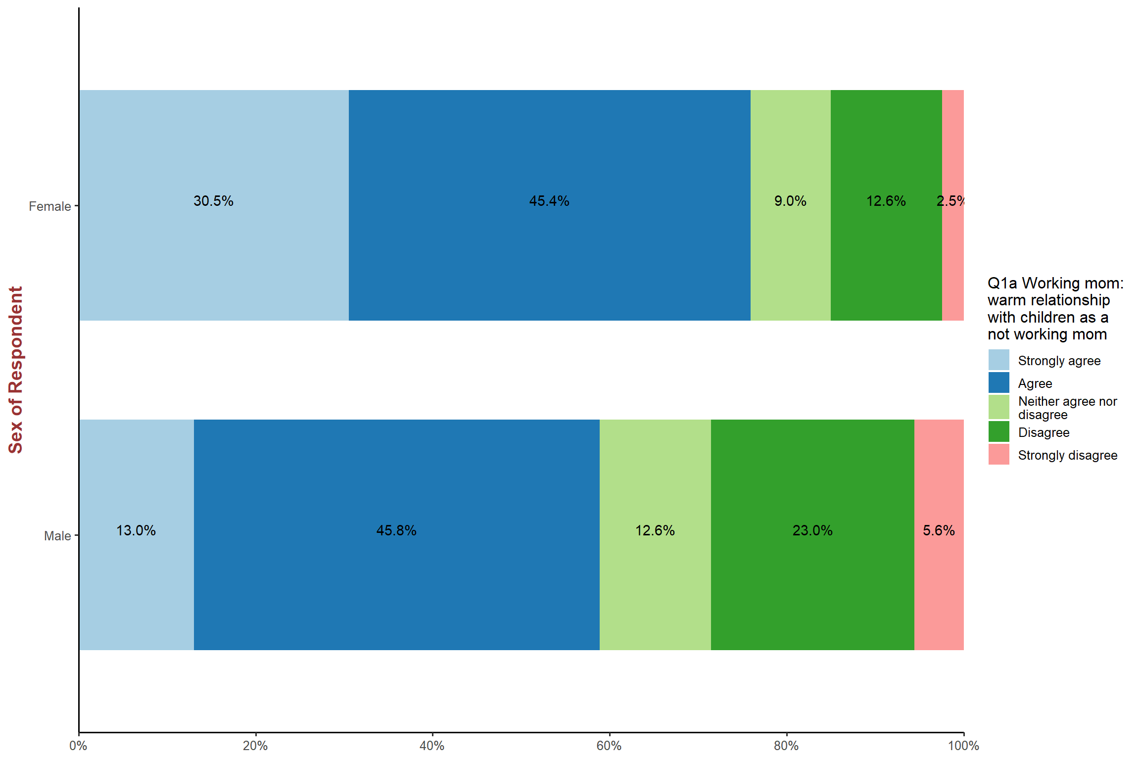
plot_xtab(aus2012$sex, aus2012$fechld, bar.pos = "stack", show.total = FALSE,
         margin = "row", coord.flip = TRUE, show.n = FALSE) + my_theme # 'margin' specifies how percentages are calculated; 'row' indicates the row percentage; 'show.n = FALSE' will remove the total number of cases.
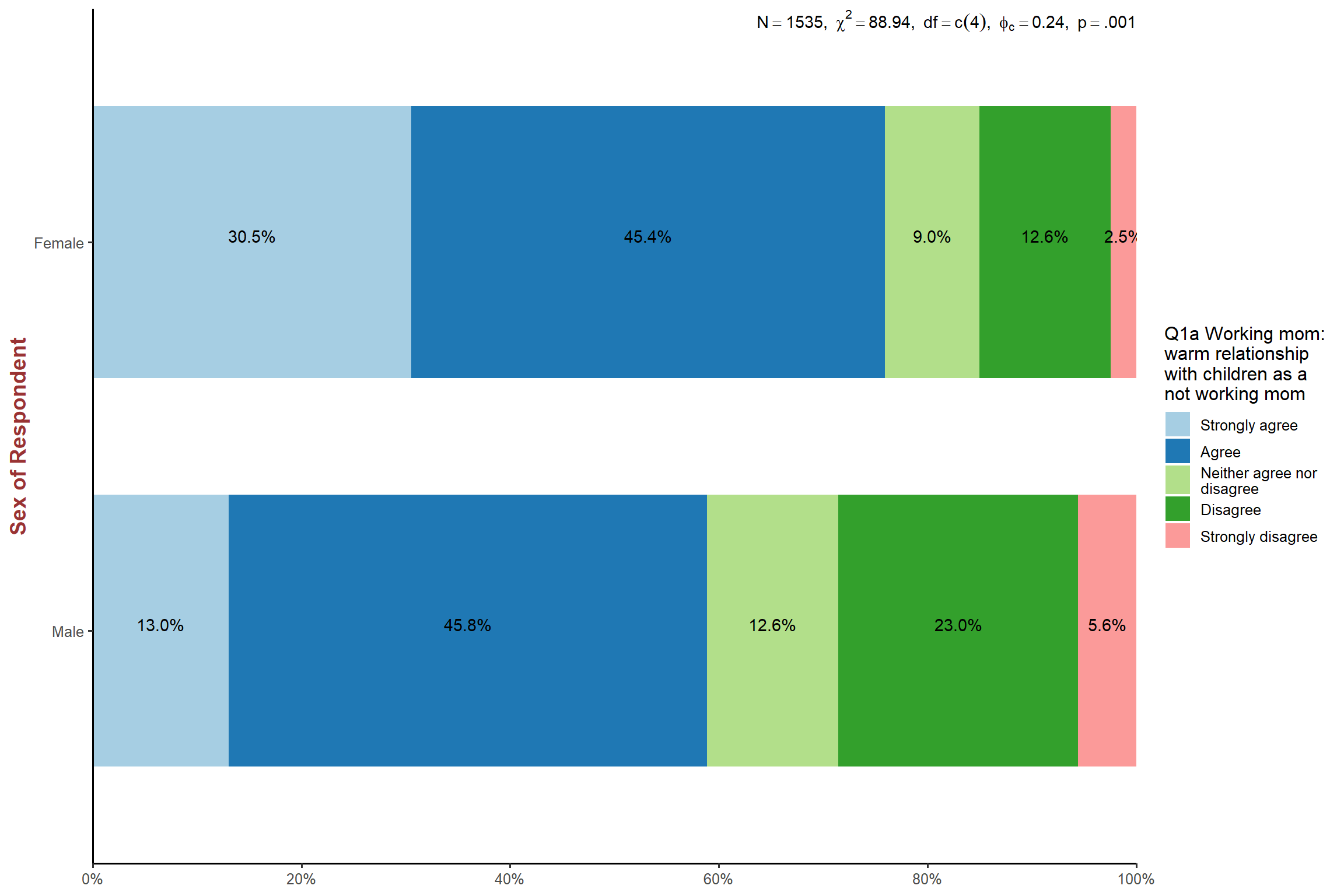
plot_xtab(aus2012$sex, aus2012$fechld, bar.pos = "stack", show.total = FALSE,
         margin = "row", coord.flip = TRUE, show.n = FALSE, show.summary = TRUE) + my_theme # show chi-square statistics
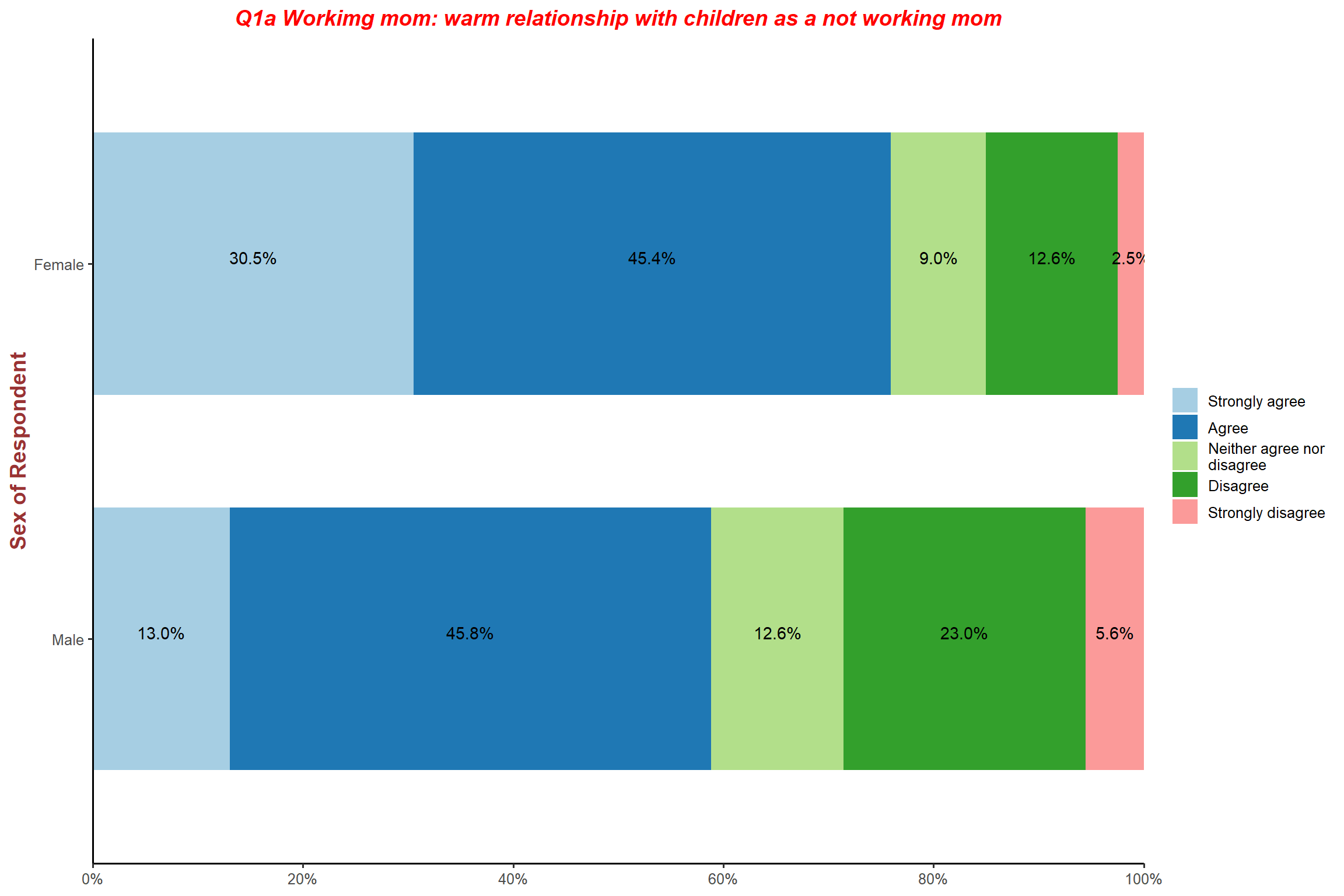
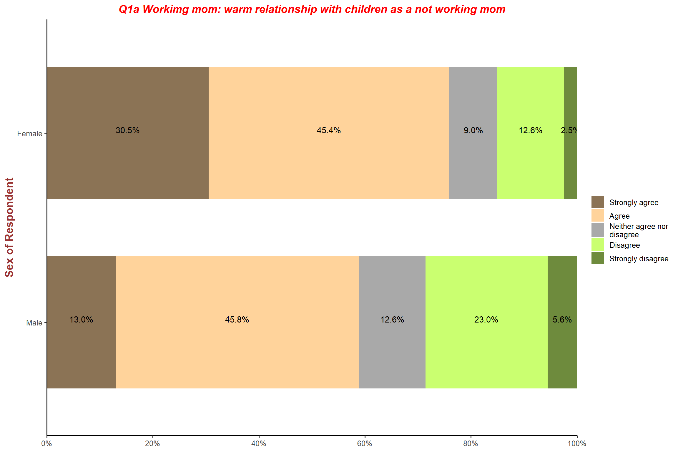
plot_xtab(aus2012$sex, aus2012$fechld, bar.pos = "stack", show.total = FALSE,
         margin = "row", coord.flip = TRUE, show.n = FALSE,
         legend.title = "",
         title = "Q1a Workimg mom: warm relationship with children as a not working mom",
         wrap.title = 70) + my_theme # remove the legend title; add the plot title; allow more characters in one line in the plot title
plot_xtab(aus2012$sex, aus2012$fechld, bar.pos = "stack", show.total = FALSE,
         margin = "row", coord.flip = TRUE, show.n = FALSE,
         legend.title = "",
         title = "Q1a Workimg mom: warm relationship with children as a not working mom",
         wrap.title = 70,
         geom.colors = c("burlywood4", "burlywood1", "darkgray", "darkolivegreen1", "darkolivegreen4")) + my_theme # change colors for each category
################################################################################
# 2. Box plot
################################################################################
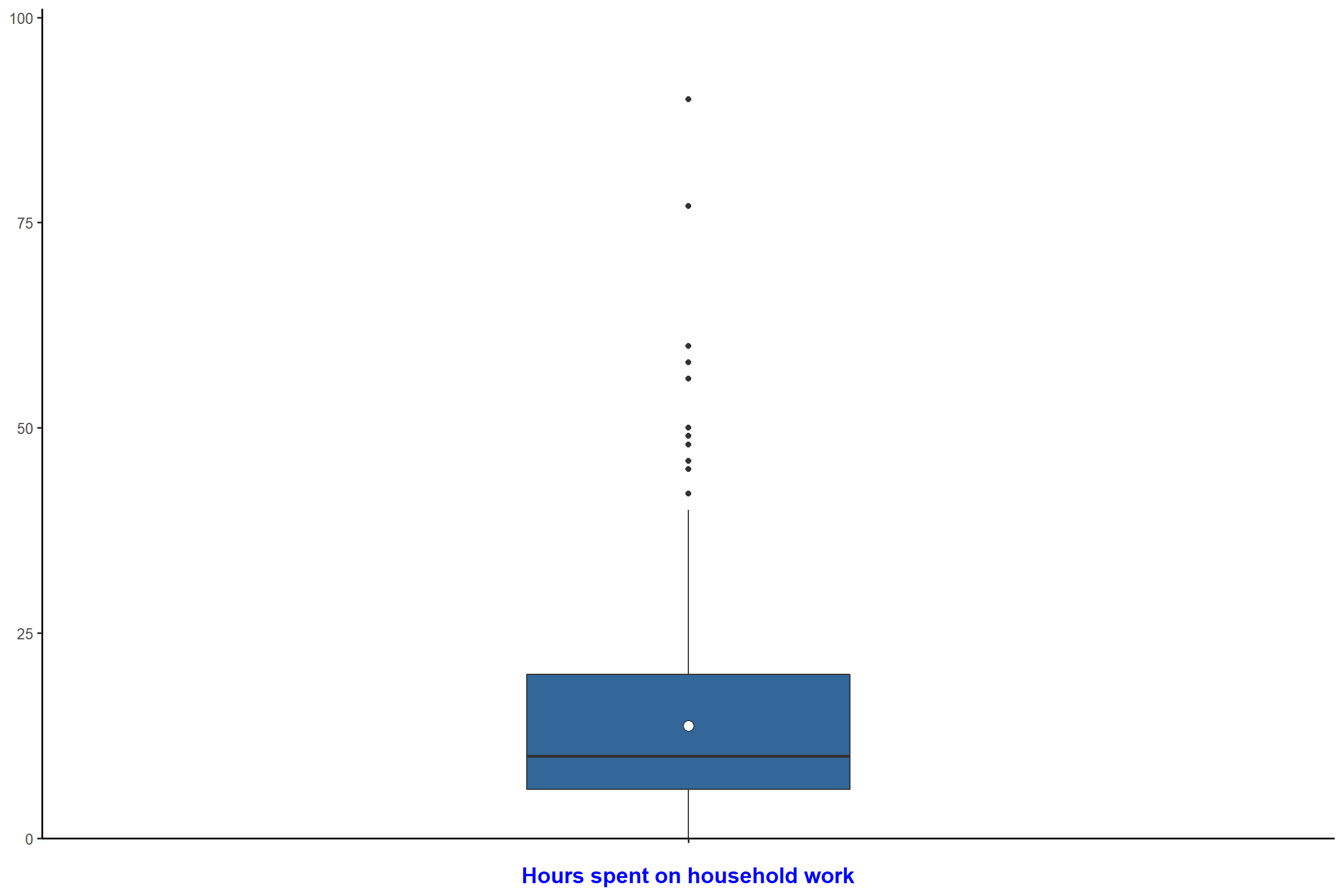
# 2.1 Simple box plot
aus2012$rhhwork <- set_label(aus2012$rhhwork, label = "Hours spent on household work") # set variable name
plot_frq(aus2012$rhhwork, type = "box") + my_theme
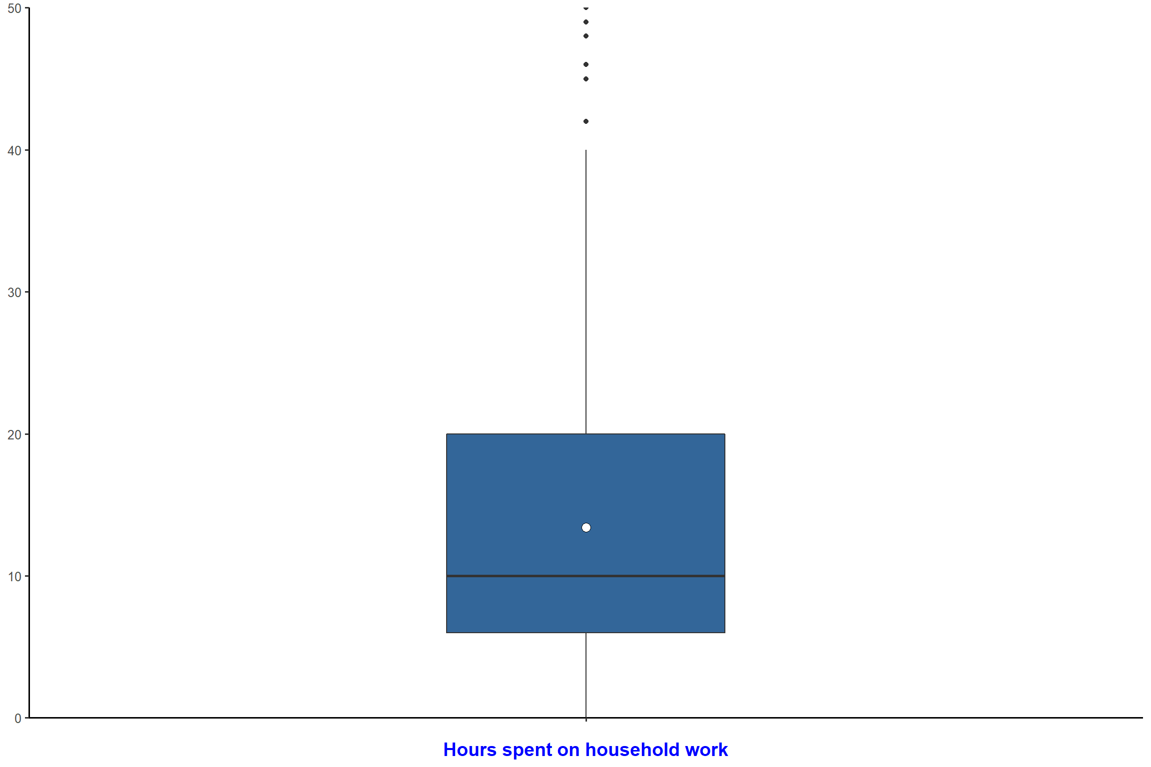
plot_frq(aus2012$rhhwork, type = "box", ylim = c(0, 50)) + my_theme # reduce the range of y-axis.
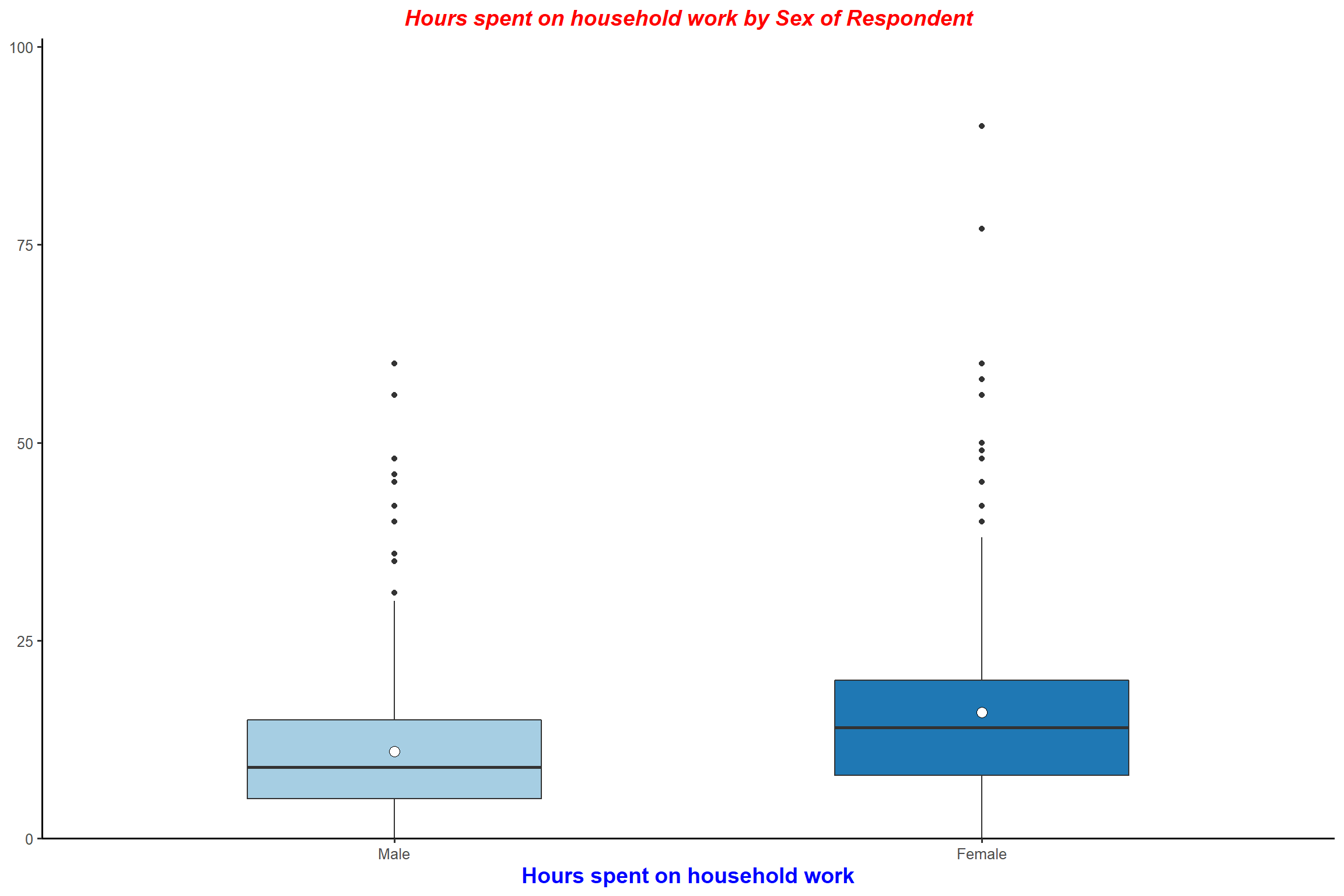
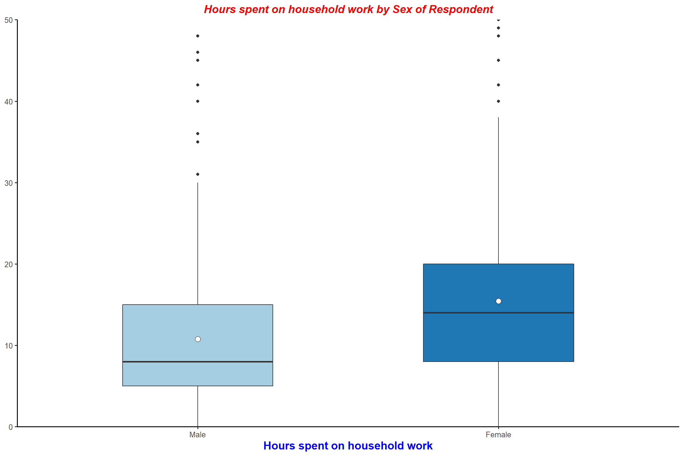
# 2.2 Grouped box plot
plot_grpfrq(aus2012$rhhwork, aus2012$sex, type = "box")  + my_theme
plot_grpfrq(aus2012$rhhwork, aus2012$sex, type = "box", ylim = c(0, 50)) + my_theme
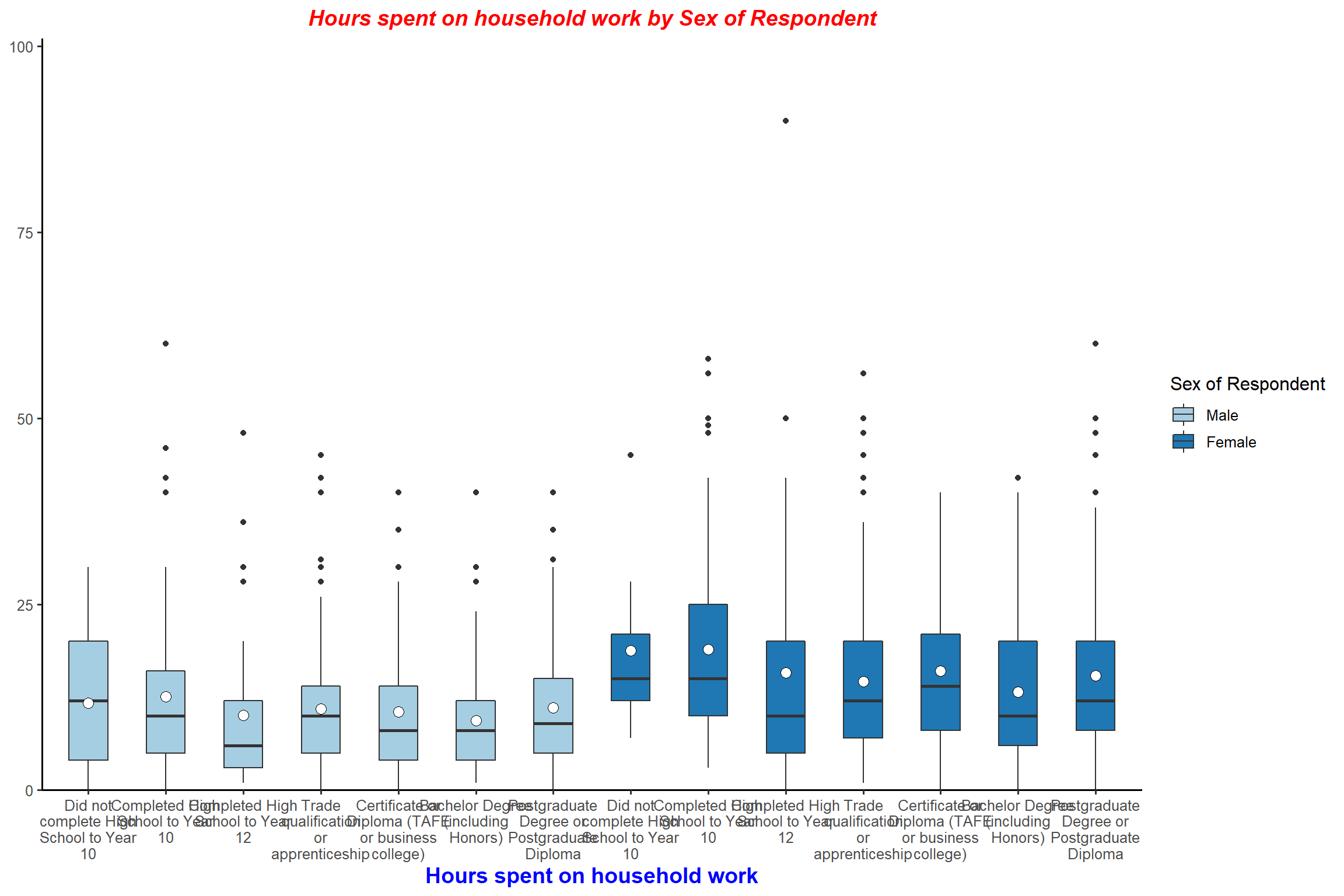
# 2.3 3-way grouped box plot
plot_grpfrq(aus2012$rhhwork, aus2012$sex, intr.var = aus2012$degree, type = "box") + my_theme # value labels are long; I will change them
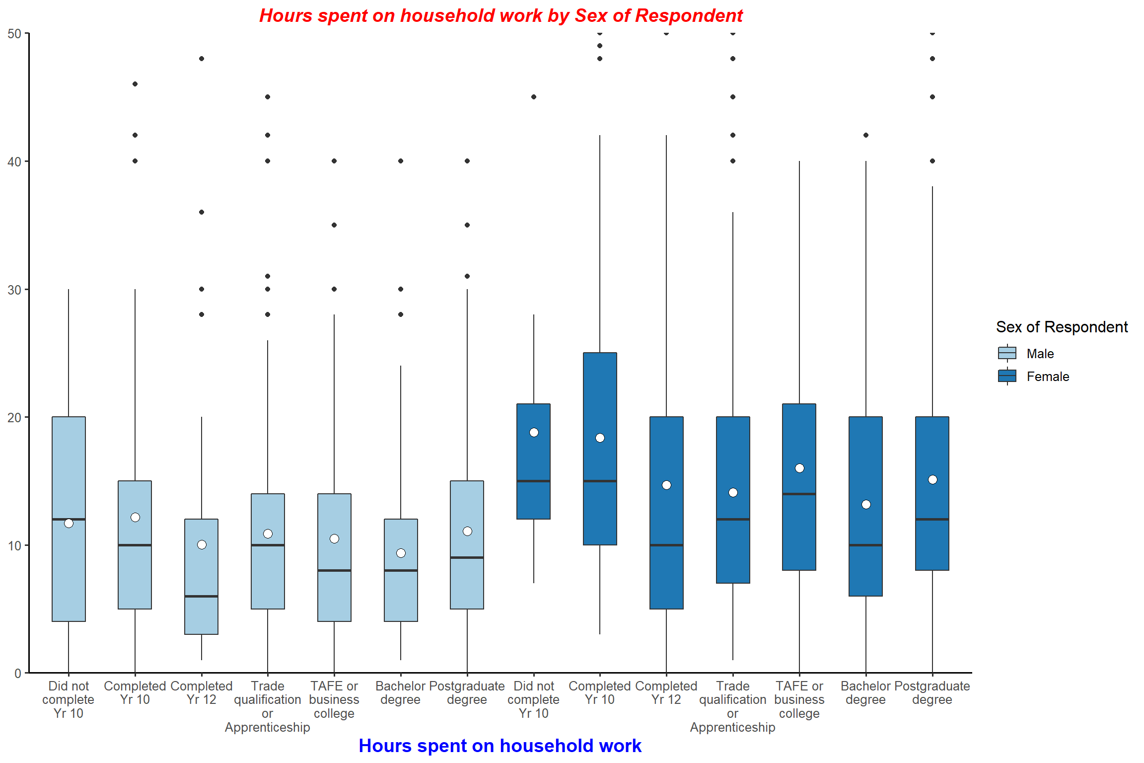
aus2012$degree <- set_labels(aus2012$degree,
                             labels = c("Did not complete Yr 10" = 1,
                                    "Completed Yr 10" = 2,
                                    "Completed Yr 12" = 3,
                                    "Trade qualification or Apprenticeship" = 4,
                                    "TAFE or business college" = 5,
                                    "Bachelor degree" = 6,
                                    "Postgraduate degree" = 7)) # reassign value labels
plot_grpfrq(aus2012$rhhwork, aus2012$sex, intr.var = aus2012$degree, type = "box",
           wrap.labels = 8, ylim = c(0, 50))  + my_theme
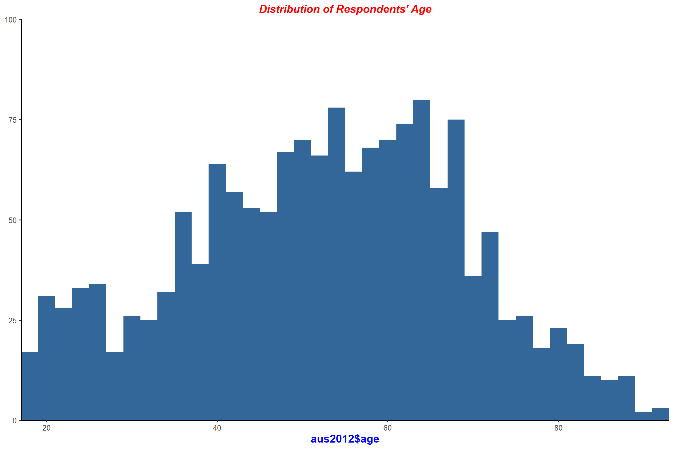
################################################################################
# 3. Histogram
################################################################################
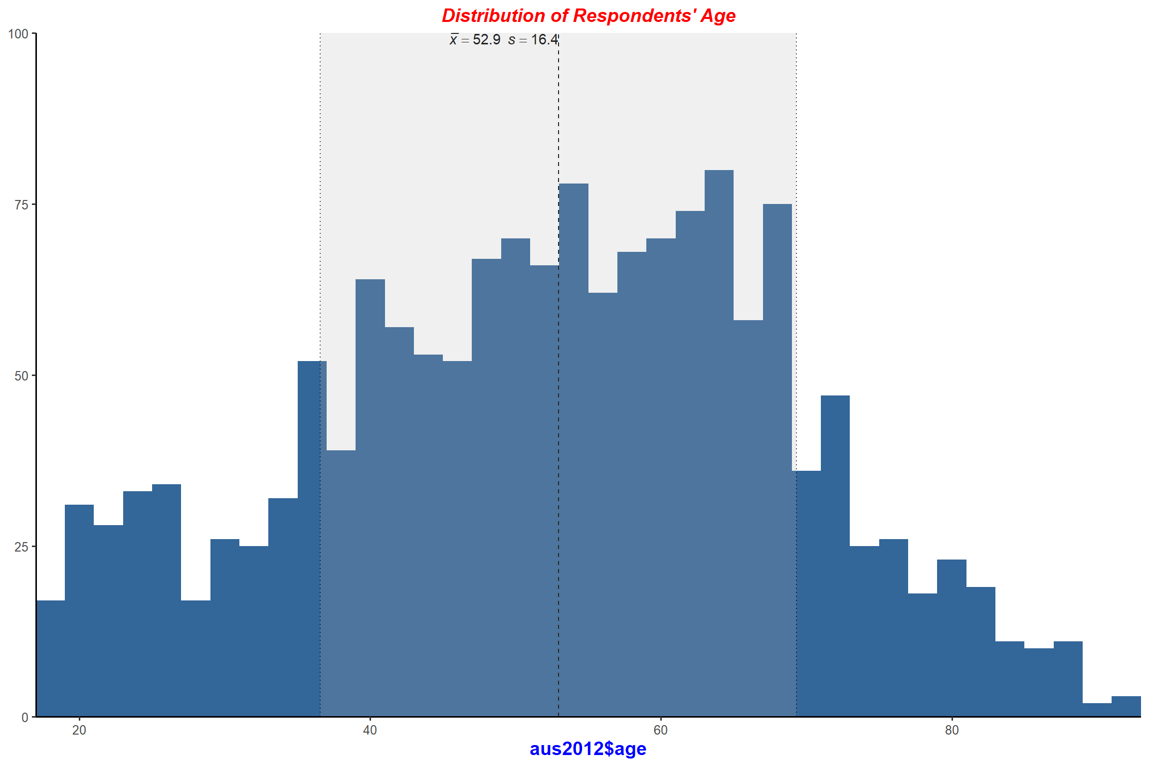
plot_frq(aus2012$age, type = "hist", title = "Distribution of Respondents' Age") + my_theme
plot_frq(aus2012$age, type = "hist", title = "Distribution of Respondents' Age",
        show.mean = TRUE) + my_theme # show mean and standard deviation
plot_frq(aus2012$age, type = "hist", title = "Distribution of Respondents' Age",
        show.mean = TRUE, normal.curve = TRUE) + my_theme # Add the normal disribution curve.

plot_frq(aus2012$age, type = "hist", title = "Distribution of Respondents' Age",
        show.mean = TRUE, normal.curve = TRUE,
        normal.curve.color = "red", normal.curve.size = 3) + my_theme # change the colour and the line width of the normal curve

################################################################################
# 4. Scatter plot
################################################################################
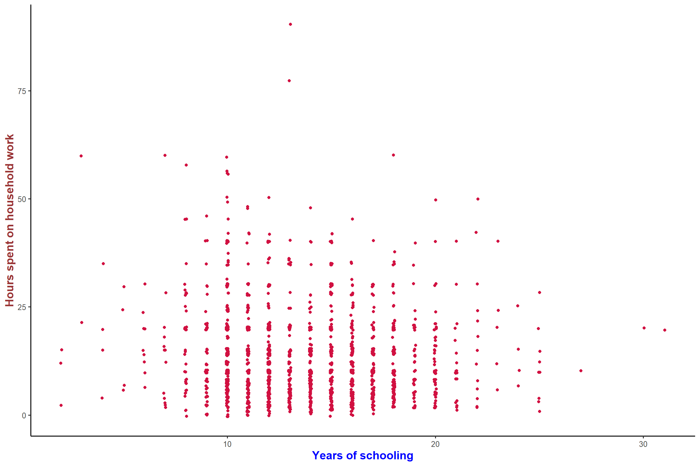
aus2012$educyrs <- set_label(aus2012$educyrs, label = "Years of schooling")
# 4.1 Simple scatter plot
plot_scatter(aus2012, educyrs, rhhwork) + my_theme
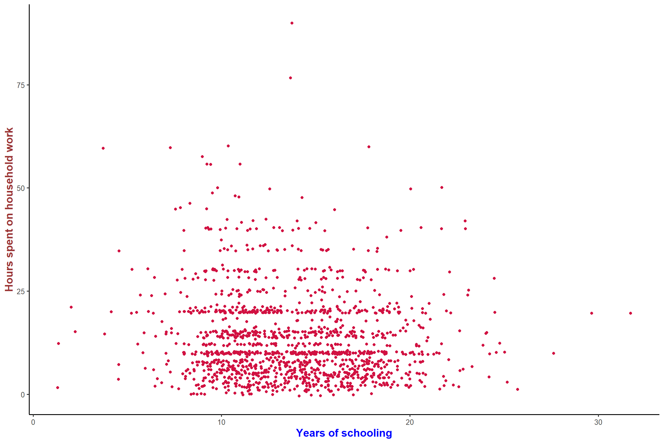
plot_scatter(aus2012, educyrs, rhhwork, jitter = TRUE)+ my_theme # points are jittered to avoid overlapping.
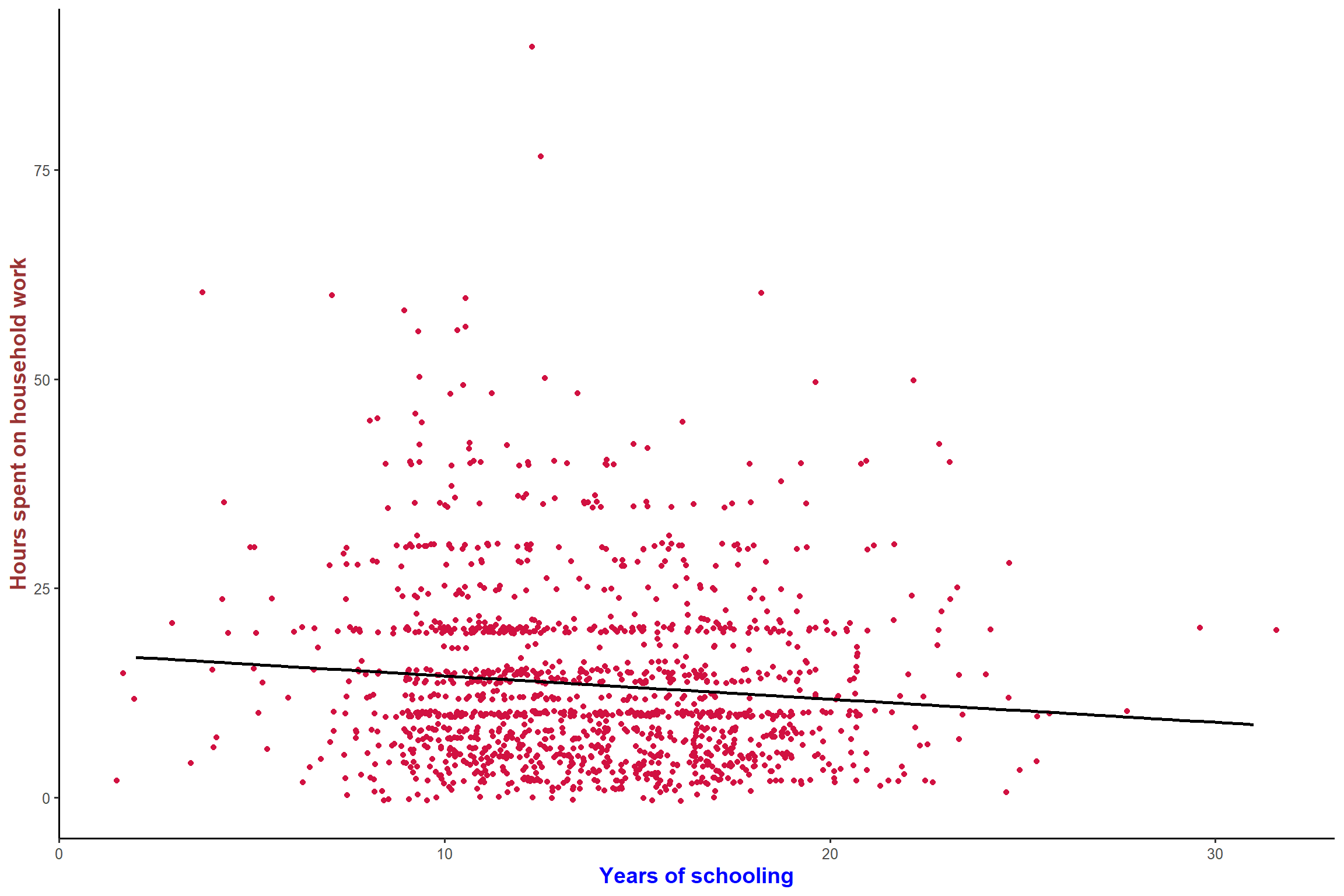
plot_scatter(aus2012, educyrs, rhhwork, jitter = TRUE, fit.line = lm)+ my_theme # add the fitted line
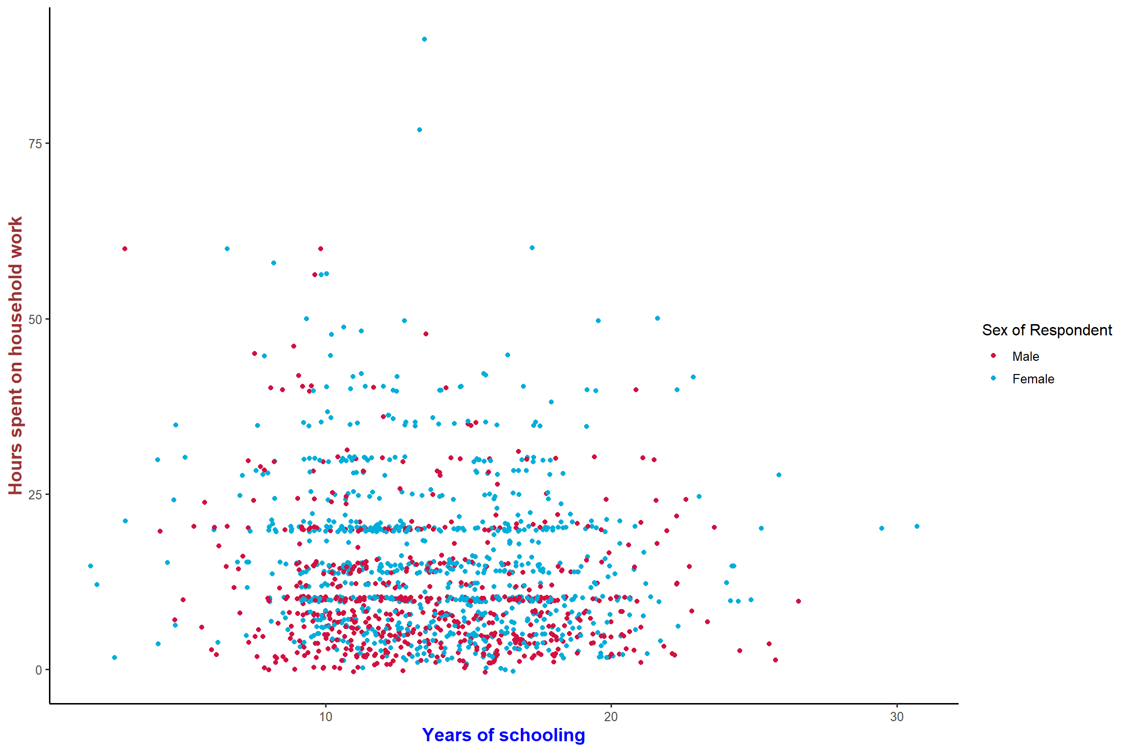
# 4.2 Grouped scatter plot
plot_scatter(aus2012, educyrs, rhhwork, sex, jitter = TRUE)+ my_theme # different colors by gender
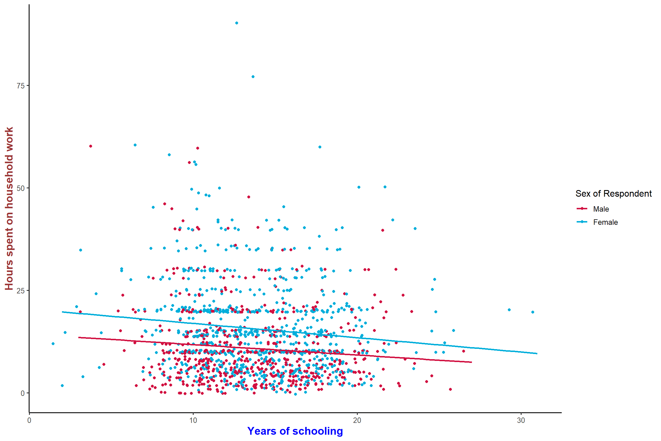
plot_scatter(aus2012, educyrs, rhhwork, sex, jitter = TRUE,
            fit.grps = lm)+ my_theme # add the fitted line for each group
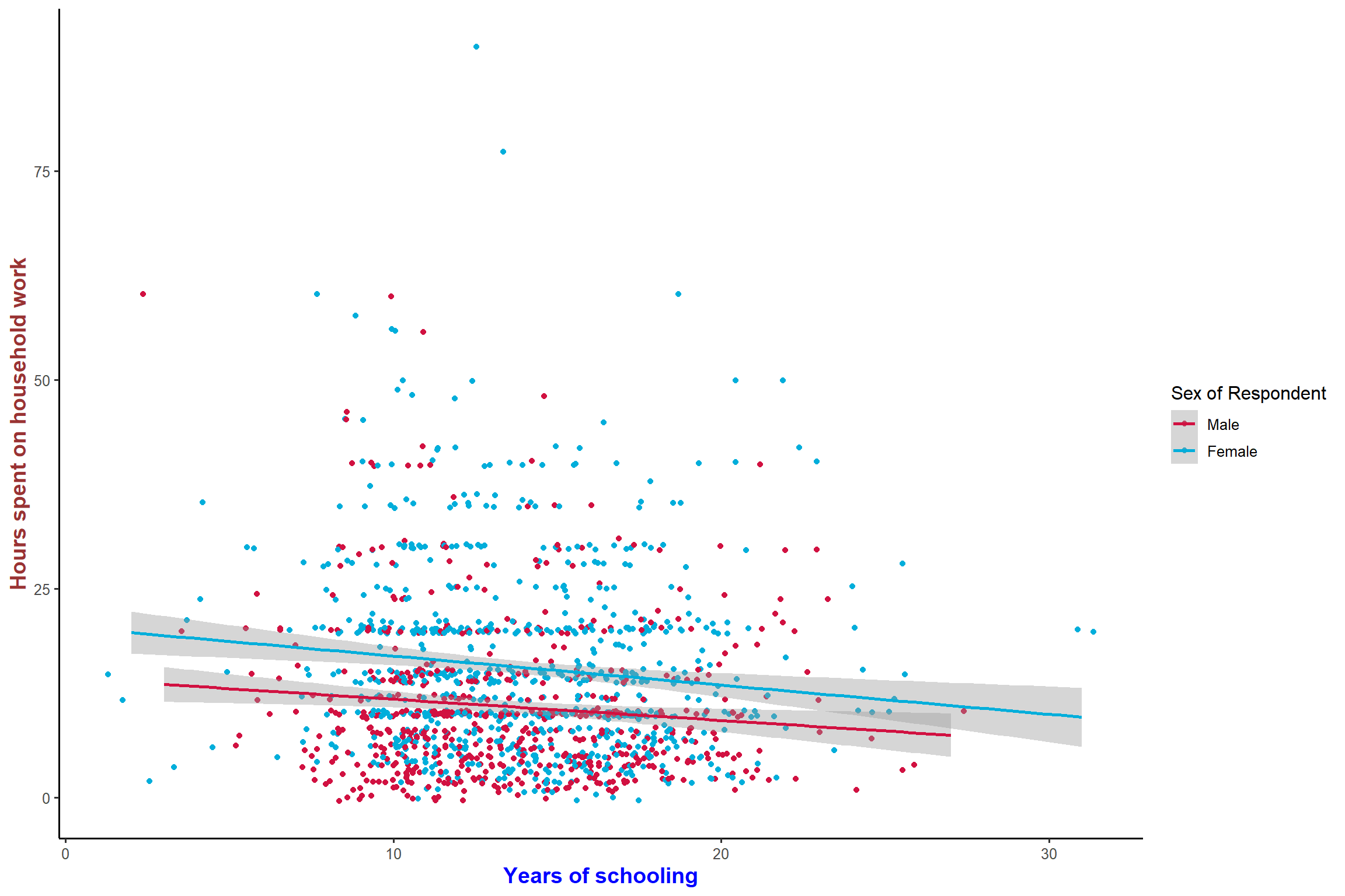
plot_scatter(aus2012, educyrs, rhhwork, sex, jitter = TRUE,
            fit.grps = lm, show.ci = TRUE)+ my_theme # show confidence intervals
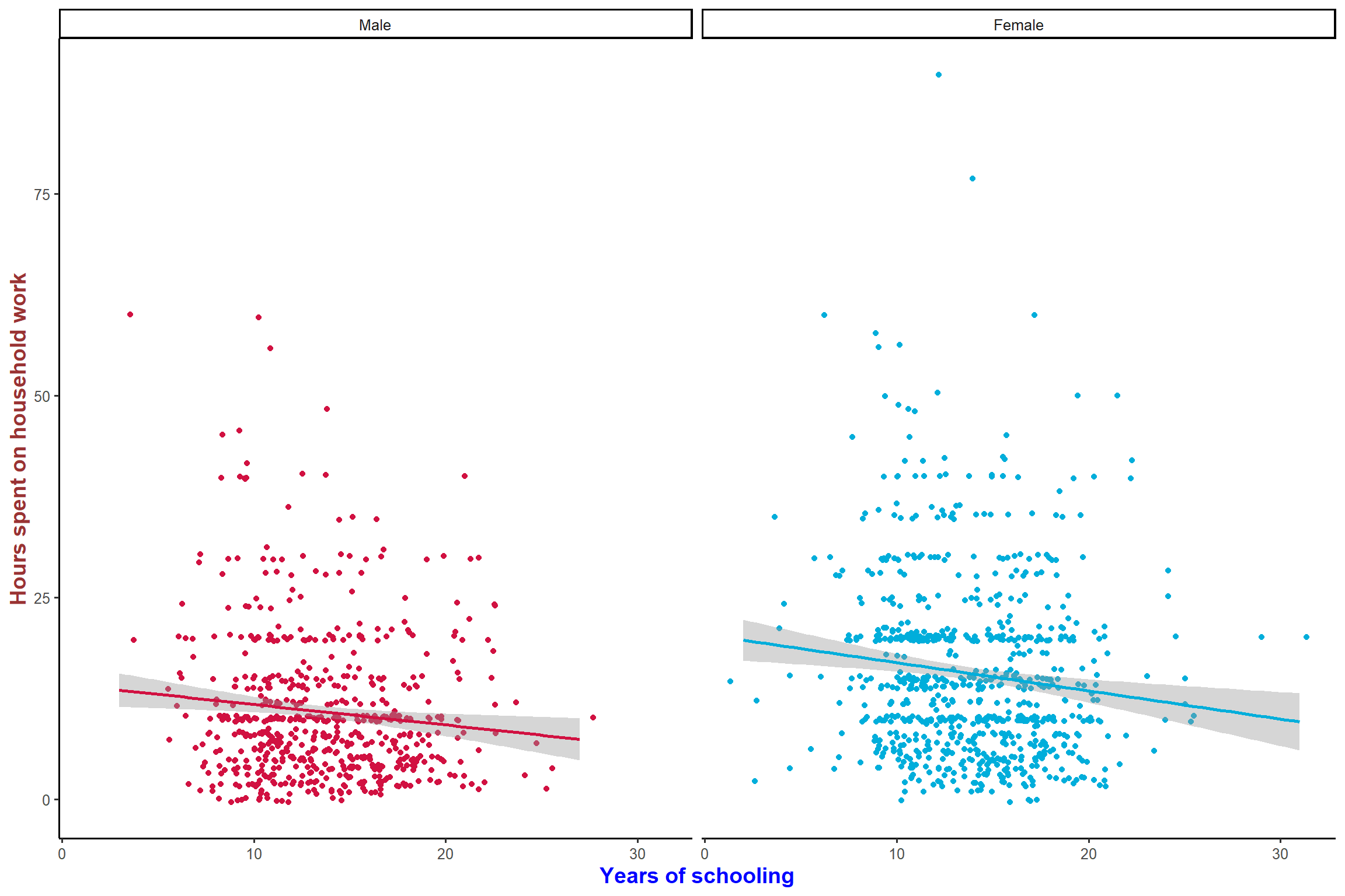
plot_scatter(aus2012, educyrs, rhhwork, sex, jitter = TRUE,
            fit.grps = lm, show.ci = TRUE, grid = TRUE)+ my_theme # grouped scatter plot as facets
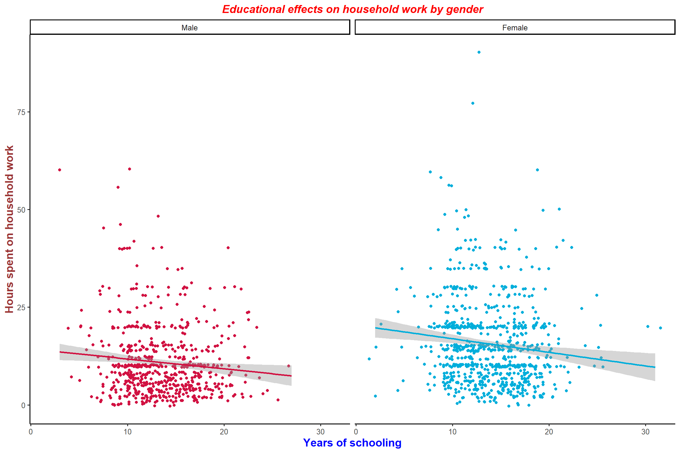
plot_scatter(aus2012, educyrs, rhhwork, sex, jitter = TRUE,
            fit.grps = lm, show.ci = TRUE, grid = TRUE,
            title = "Educational effects on household work by gender")+ my_theme # add the title
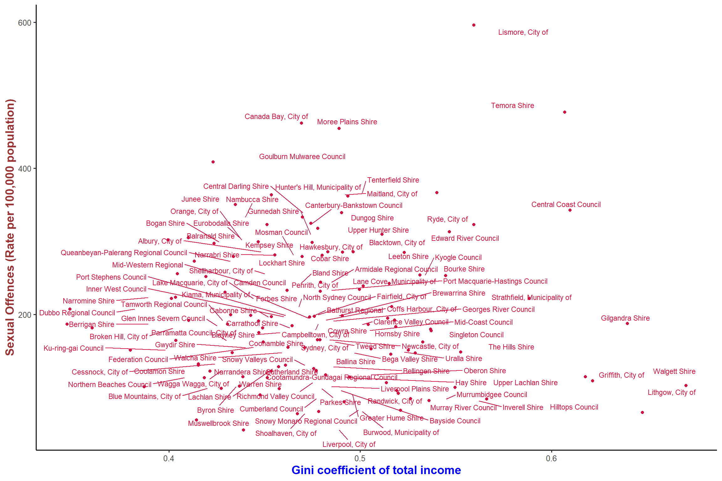
# 4.3 Scatter plot with text label
plot_scatter(lga, giniinc, sexoff, dot.labels = lga$name3)+ my_theme #This is too busy
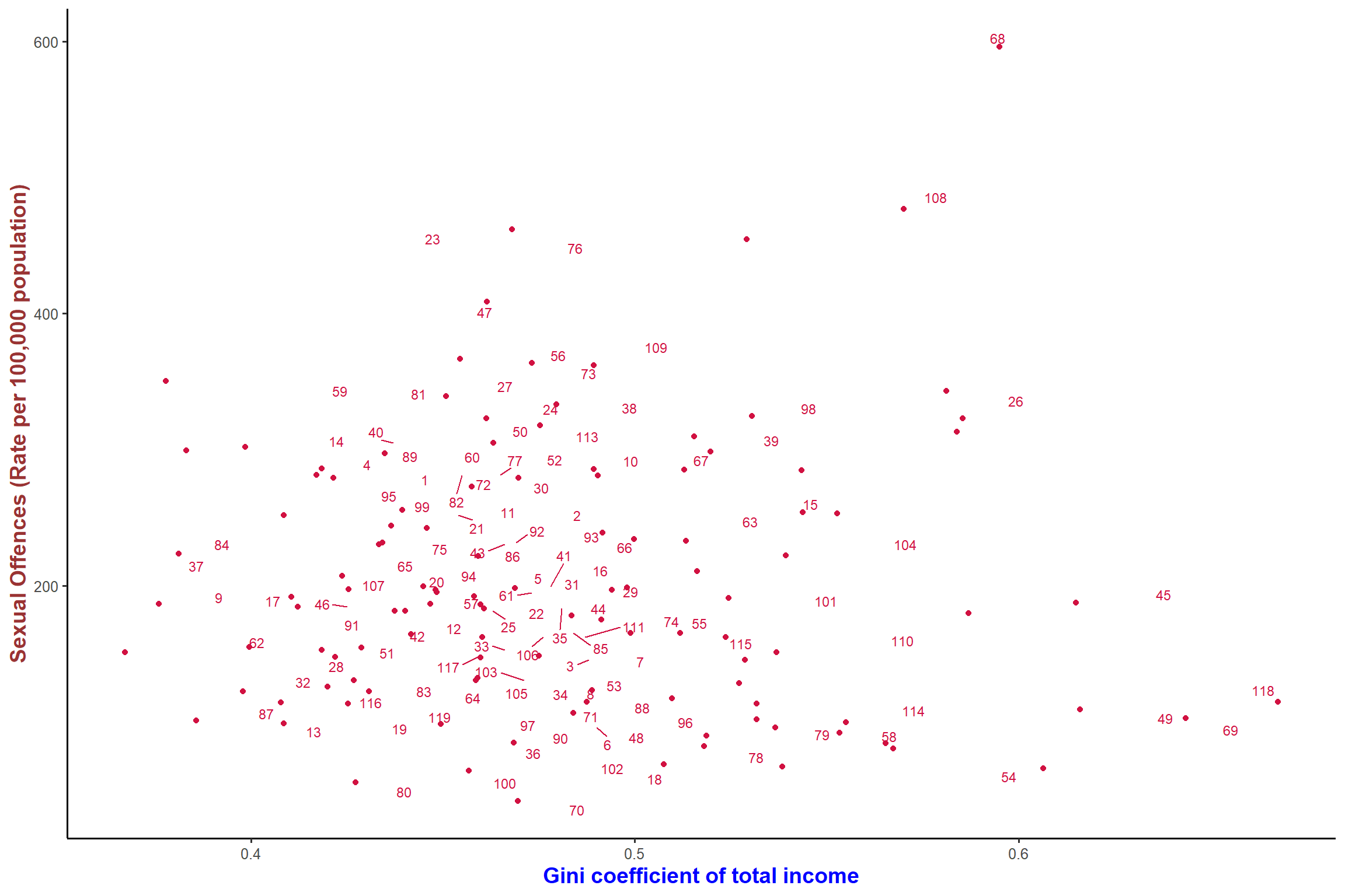
plot_scatter(lga, giniinc, sexoff, dot.labels = lga$name) + my_theme
################################################################################
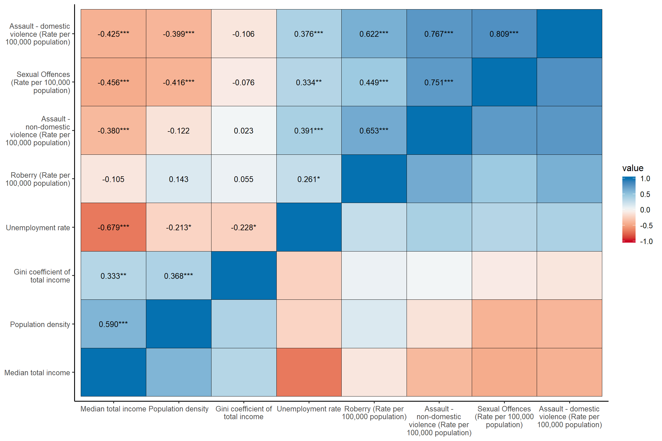
# 5. Correlation matrix
################################################################################
var.index <- c("astdomviol", "astnondomviol", "sexoff", "robbery", "popden", "medinc", "giniinc", "unemploy") # make a list of variables for correlation matrix
sjp.corr(lga[,var.index]) + my_theme
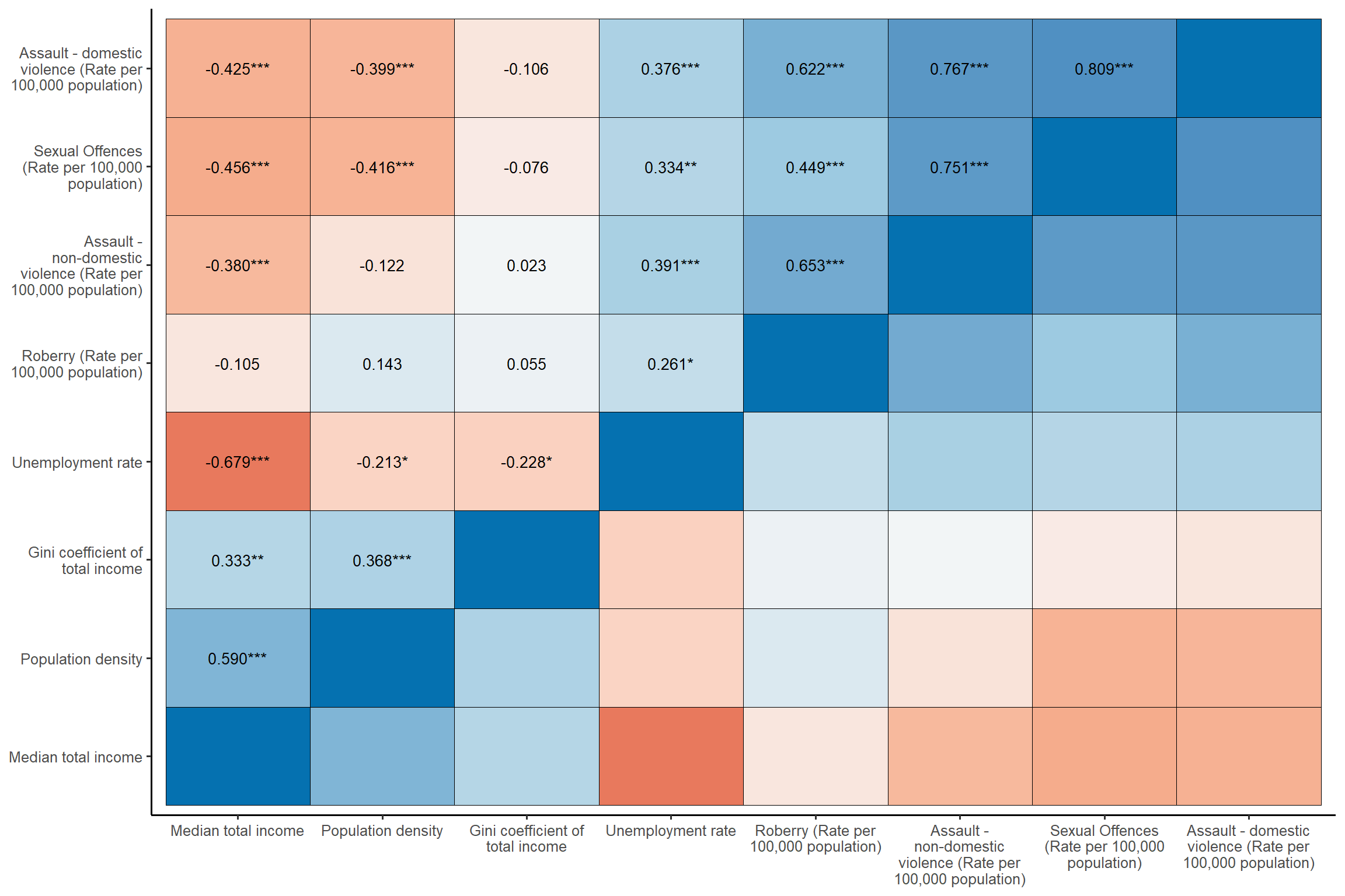
sjp.corr(lga[,var.index], show.legend = TRUE)+ my_theme # show the legend for colours
################################################################################
# 6. Regression
################################################################################
# data preparation
var.list <- c("fepresch", "famsuffr","rhhwork", "educyrs", "sex", "work", "topbot", "age", "marital", "id", "risei") # select variables.
mydata <- aus2012[, var.list] # make a dataset with the chosen variables
#------------
# In the next section the dplyr operator %>% is used.
# For an introduction to the %>% operator see this:
# https://cran.r-project.org/web/packages/magrittr/vignettes/magrittr.html
#------------
mydata <- mydata %>%
            select(marital) %>%
            rec(rec = "1:2 = 1; 3:6 = 0") %>% # old value = new value; 3:6 means 3 to 6.
            add_columns(mydata) # recode 'marital' in a way that those currently married or in a partnership are coded as 1, otherwise as 0.
mydata <- mydata %>%
            select(marital_r) %>%
            to_factor() %>%
            add_columns(mydata) # convert the variable into a factor
mydata <- mydata %>%
            rename(currmarried = marital_r) # change the variable name into 'currmarried'.
#------------
mydata <- mydata %>%
            select(sex) %>%
            to_dummy() %>%
            add_columns(mydata) # make dummy variables for sex
mydata <- mydata %>%
            rename(male = sex_1, female = sex_2) # change the variable names
mydata <- mydata %>%
            select(male, female) %>%
            to_factor() %>%
            add_columns(mydata) # convert the variables into factors.
#------------
mydata <- mydata %>%
          select(work) %>%
          to_dummy() %>%
          add_columns(mydata) # make dummy variables for work
mydata <- mydata %>%
  rename(currwrk = work_1, pastwrk = work_2, nowrk = work_3) # change the variable names
mydata <- mydata %>%
  select(currwrk, pastwrk, nowrk) %>%
  to_factor() %>%
  add_columns(mydata) # convert the variables into factors.
#------------
mydata <- mydata %>%
          select(fepresch, famsuffr) %>%
          dicho(dich.by = 3) %>%
          add_columns(mydata) # 'disagree" and "strongly disagree" are collapsed into 1, otherwise 0
mydata <- mydata %>%
  select(fepresch_d, famsuffr_d) %>%
  to_factor() %>%
  add_columns(mydata) # convert the variables into factors.
#------------
mydata$female <- set_label(mydata$female, label = "Female")
mydata$female <- set_labels(mydata$female, labels = c("Male"= 0, "Female" = 1))
mydata$currmarried <- set_label(mydata$currmarried, label = "Currently married or in a partnership")
mydata$age <- set_label(mydata$age, label = "Age")
mydata$educyrs <- set_label(mydata$educyrs, label = "Years of schooling")
mydata$topbot <- set_label(mydata$topbot, label = "Class")
mydata$currwrk <- set_label(mydata$currwrk, label = "Currently working")
mydata$rhhwork <- set_label(mydata$rhhwork, label = "Hours spent on household working")
mydata$fepresch_d <- set_label(mydata$fepresch_d, label ="Attitude toward working mom: disagree with the statement that preschool child is likely to suffer.")
#------------
################################################################################
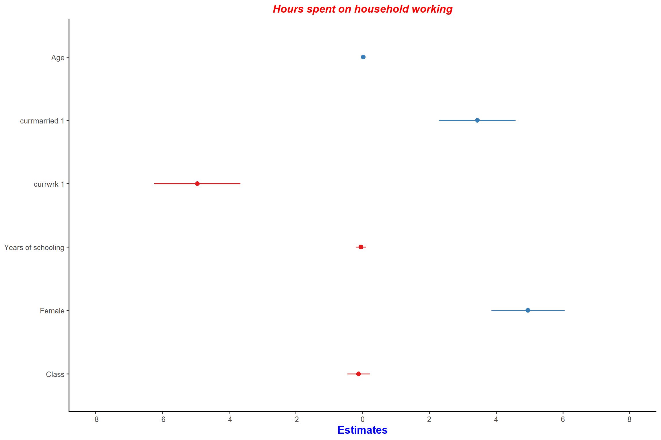
# 6.1 lm model - OLS regression model
mod1 <- lm(rhhwork ~ educyrs + age + topbot + female + currmarried + currwrk, data = mydata)
summary(mod1)
##
## Call:
## lm(formula = rhhwork ~ educyrs + age + topbot + female + currmarried +
##     currwrk, data = mydata)
##
## Residuals:
##    Min     1Q Median     3Q    Max
## -20.59  -6.36  -1.75   4.22  73.63
##
## Coefficients:
##              Estimate Std. Error t value Pr(>|t|)
## (Intercept)   12.0120     2.0146    5.96  3.2e-09 ***
## educyrs       -0.0493     0.0775   -0.64     0.52
## age            0.0212     0.0205    1.03     0.30
## topbot        -0.1146     0.1702   -0.67     0.50
## female1        4.9572     0.5581    8.88  < 2e-16 ***
## currmarried1   3.4371     0.5864    5.86  5.9e-09 ***
## currwrk1      -4.9496     0.6559   -7.55  8.6e-14 ***
## ---
## Signif. codes:  0 '***' 0.001 '**' 0.01 '*' 0.05 '.' 0.1 ' ' 1
##
## Residual standard error: 9.69 on 1253 degrees of freedom
##   (352 observations deleted due to missingness)
## Multiple R-squared:  0.141,  Adjusted R-squared:  0.137
## F-statistic: 34.3 on 6 and 1253 DF,  p-value: <2e-16
mod2 <- lm(rhhwork ~ age + educyrs * female, data = mydata)
summary(mod2)
##
## Call:
## lm(formula = rhhwork ~ age + educyrs * female, data = mydata)
##
## Residuals:
##    Min     1Q Median     3Q    Max
## -19.88  -6.62  -2.25   4.04  76.89
##
## Coefficients:
##                 Estimate Std. Error t value Pr(>|t|)
## (Intercept)       5.4779     1.9227    2.85   0.0044 **
## age               0.1203     0.0175    6.90    8e-12 ***
## educyrs          -0.0929     0.1066   -0.87   0.3837
## female1           6.3706     2.0144    3.16   0.0016 **
## educyrs:female1  -0.0788     0.1411   -0.56   0.5767
## ---
## Signif. codes:  0 '***' 0.001 '**' 0.01 '*' 0.05 '.' 0.1 ' ' 1
##
## Residual standard error: 10 on 1422 degrees of freedom
##   (185 observations deleted due to missingness)
## Multiple R-squared:  0.0917, Adjusted R-squared:  0.0891
## F-statistic: 35.9 on 4 and 1422 DF,  p-value: <2e-16
# Forest plot (coefficient and its confidence intervals)
plot_model(mod1, type = "est") + my_theme
plot_model(mod1, type = "est", remove.estimates = c("educyrs", "age", "topbot"))+ my_theme # remove estimates for 'educyrs", "age' and "topbot'

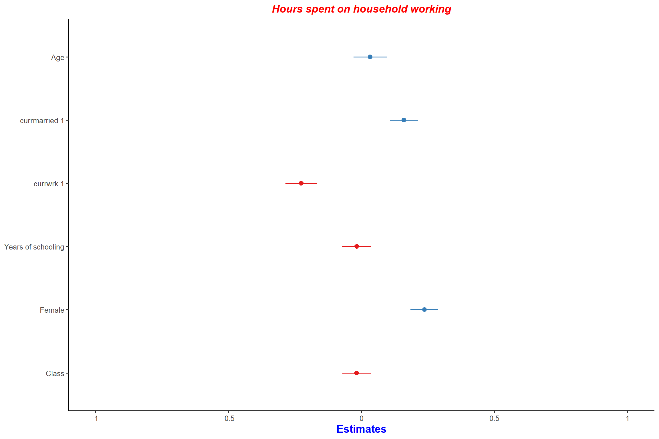
plot_model(mod1, type = "std") + my_theme # forest-plot with standardized coefficients
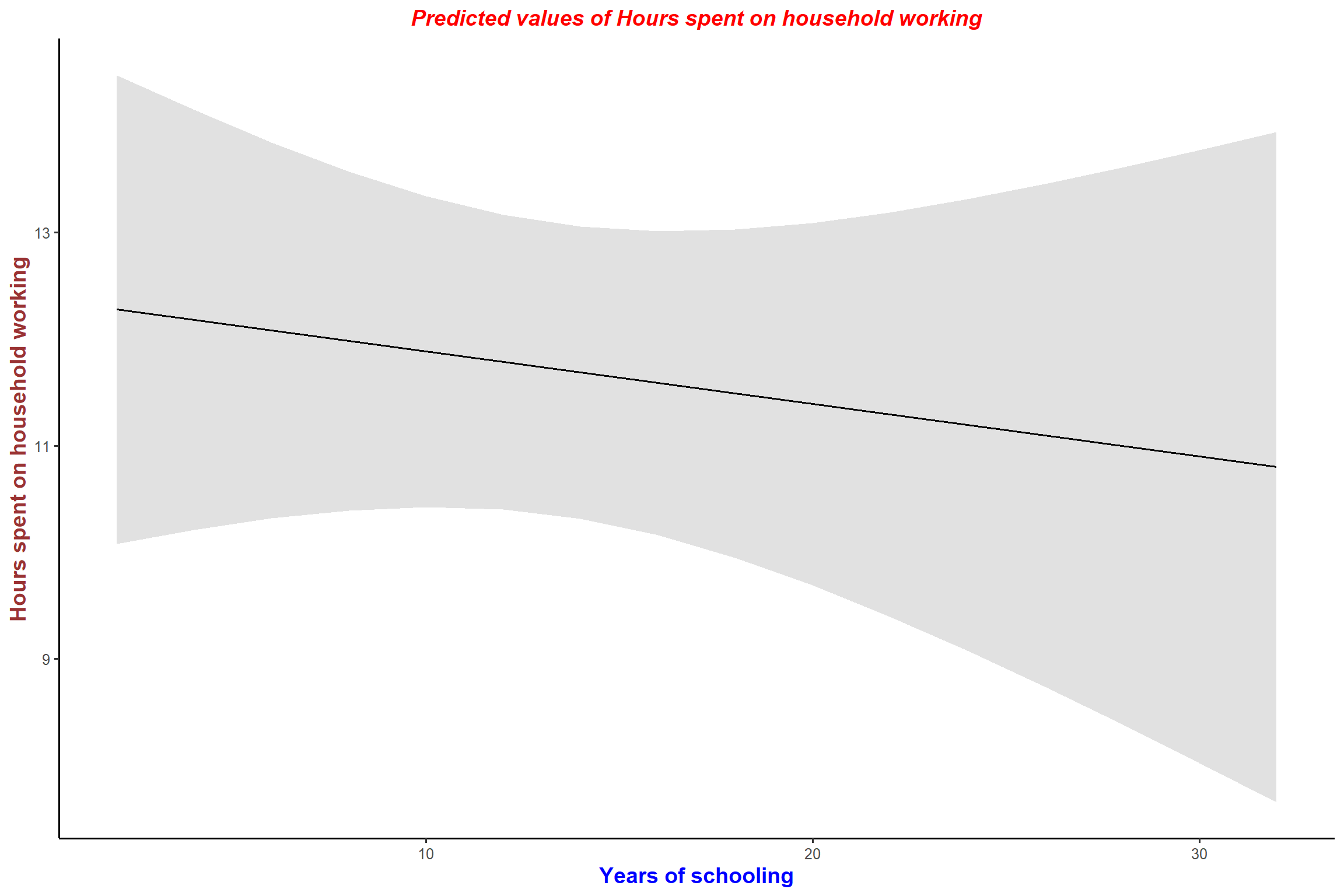
# Plot predicted values
plot_model(mod1, type = "pred", terms = "educyrs") + my_theme
plot_model(mod1, type = "pred", terms = "female") + my_theme
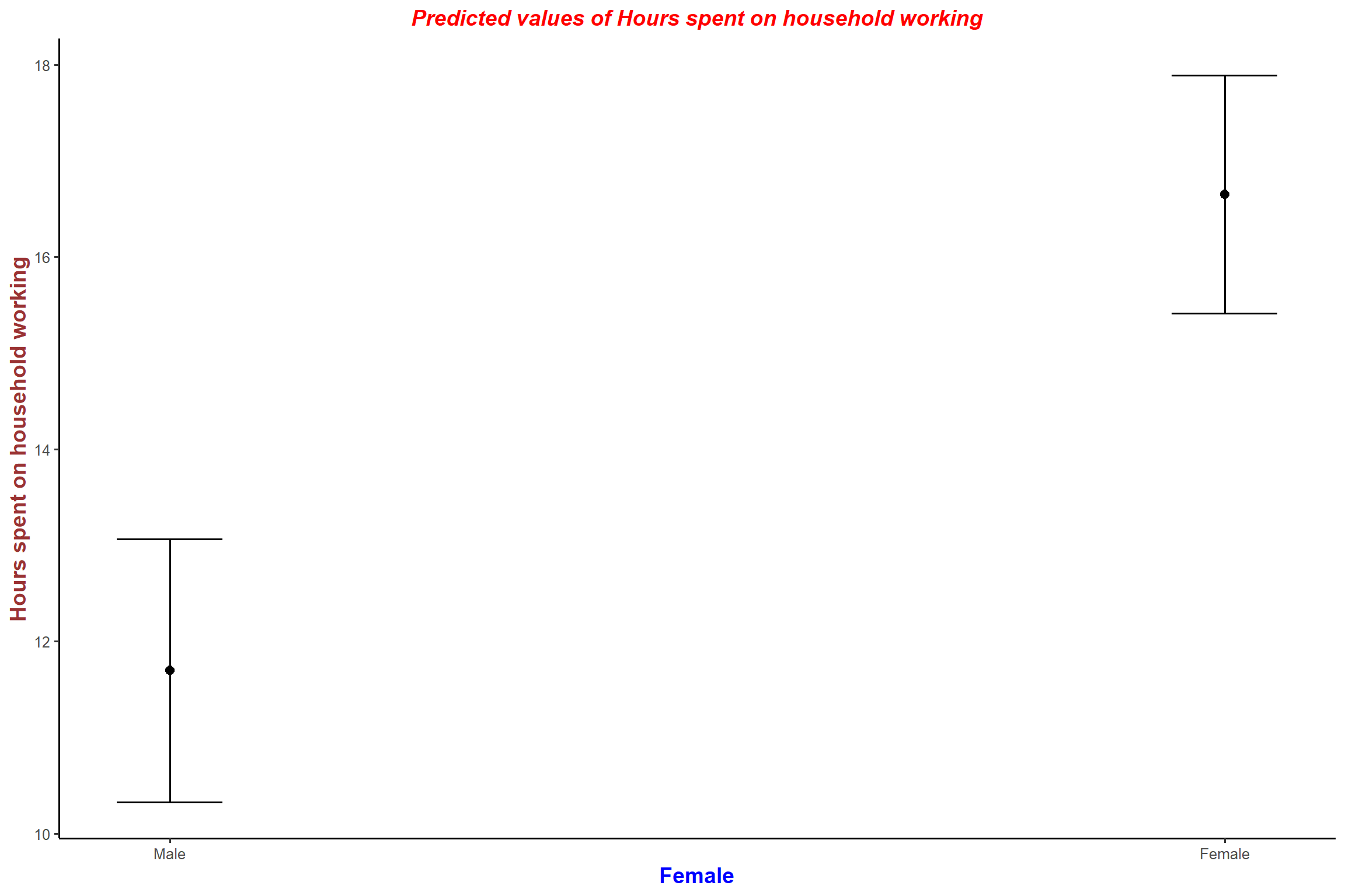
plot_model(mod1, type = "pred", terms = "female", geom.size = 1.1)+ my_theme # increase the width of the fitted line

# Plot interaction effect
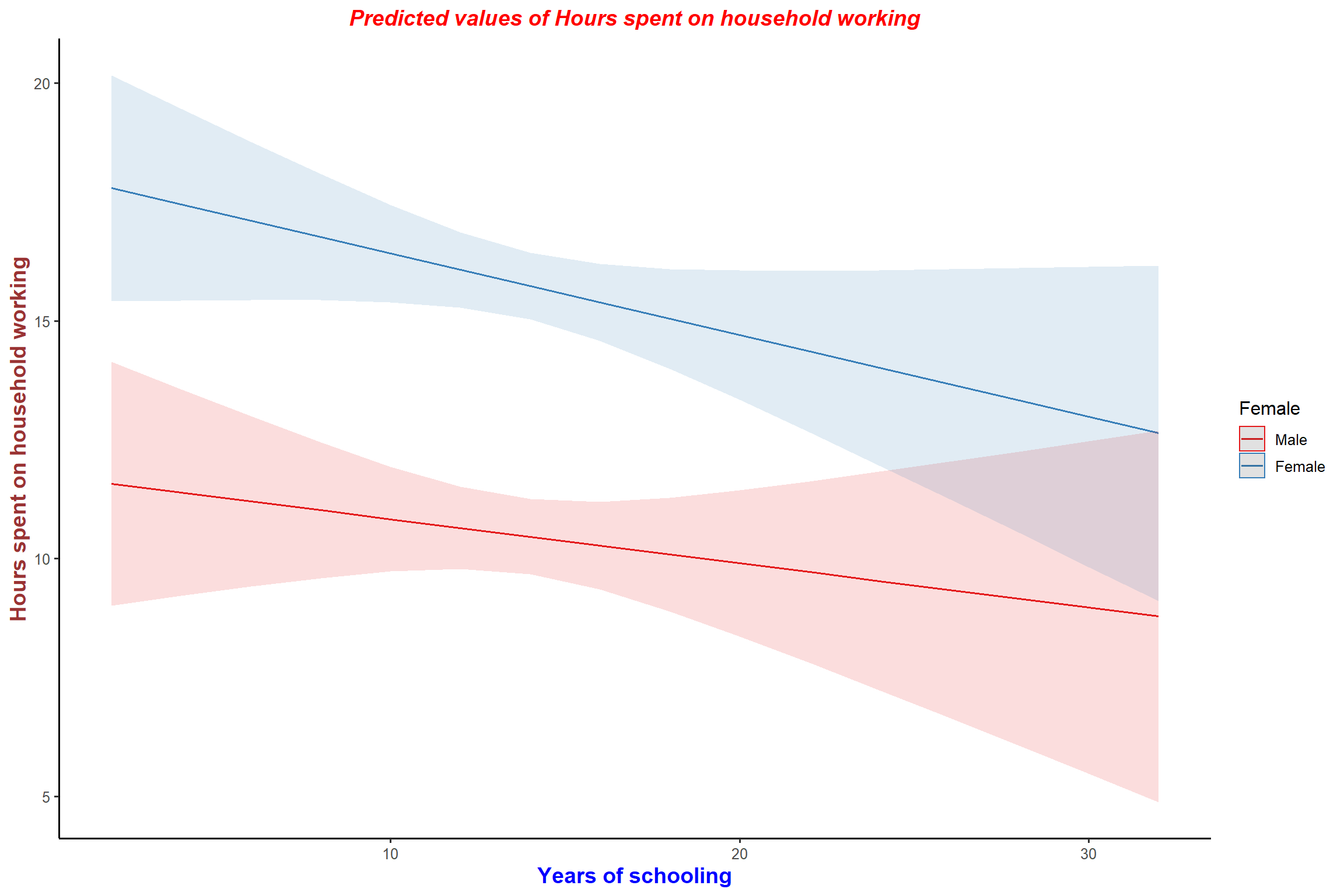
plot_model(mod2, type = "int") + my_theme
################################################################################
# 6.2 glm model - logistic regression
################################################################################
# logit model
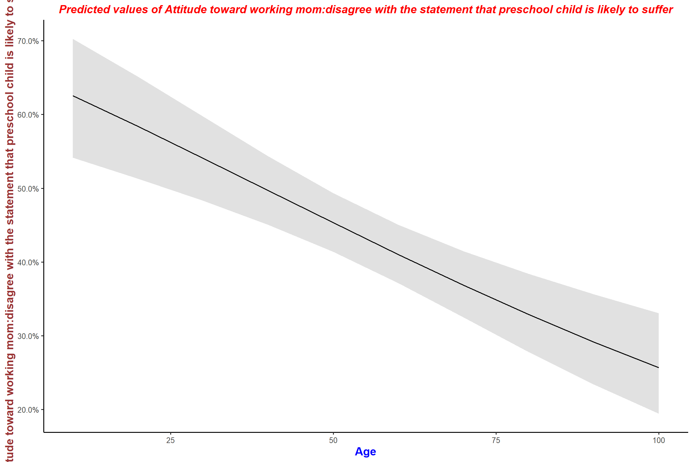
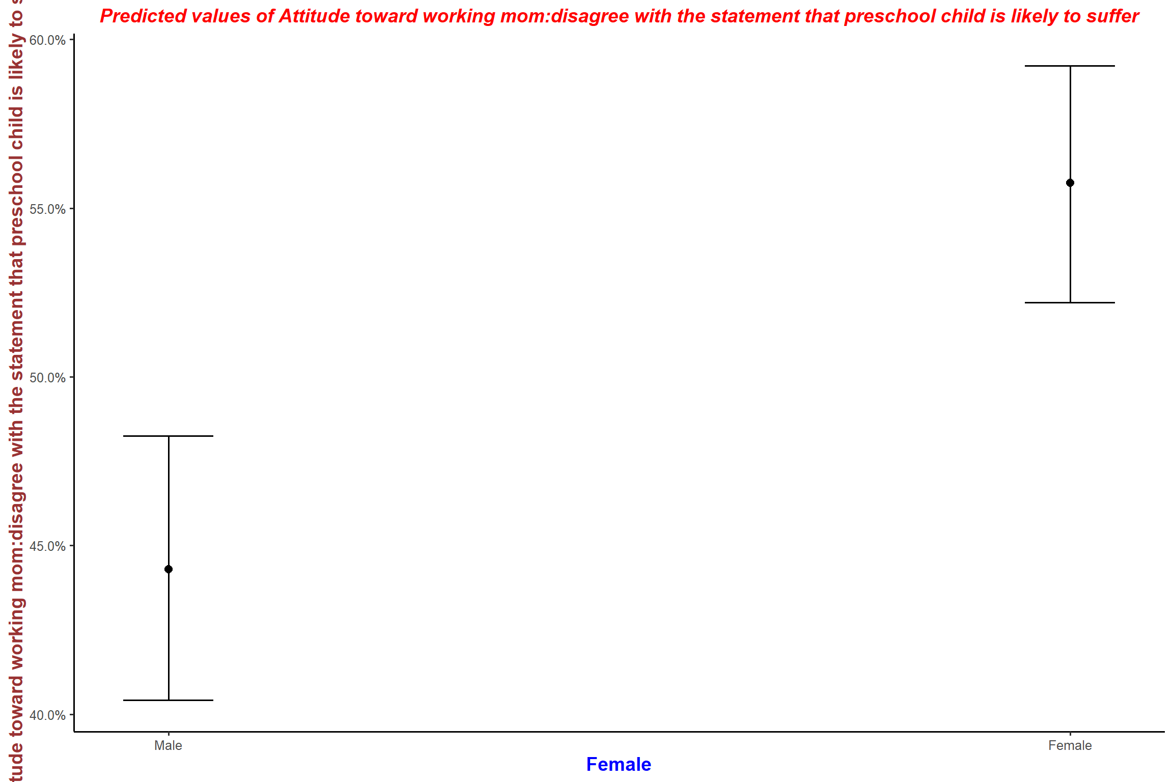
mod3 <- glm(fepresch_d ~ age + educyrs + female, data = mydata, family = "binomial")
summary(mod3)
##
## Call:
## glm(formula = fepresch_d ~ age + educyrs + female, family = "binomial",
##     data = mydata)
##
## Deviance Residuals:
##    Min      1Q  Median      3Q     Max
## -1.665  -1.141   0.819   1.119   1.670
##
## Coefficients:
##             Estimate Std. Error z value   Pr(>|z|)
## (Intercept)  0.03572    0.32999    0.11     0.9138
## age         -0.01753    0.00357   -4.91 0.00000089 ***
## educyrs      0.04750    0.01502    3.16     0.0016 **
## female1      0.45978    0.10924    4.21 0.00002565 ***
## ---
## Signif. codes:  0 '***' 0.001 '**' 0.01 '*' 0.05 '.' 0.1 ' ' 1
##
## (Dispersion parameter for binomial family taken to be 1)
##
##     Null deviance: 2001.6  on 1443  degrees of freedom
## Residual deviance: 1926.7  on 1440  degrees of freedom
##   (168 observations deleted due to missingness)
## AIC: 1935
##
## Number of Fisher Scoring iterations: 4
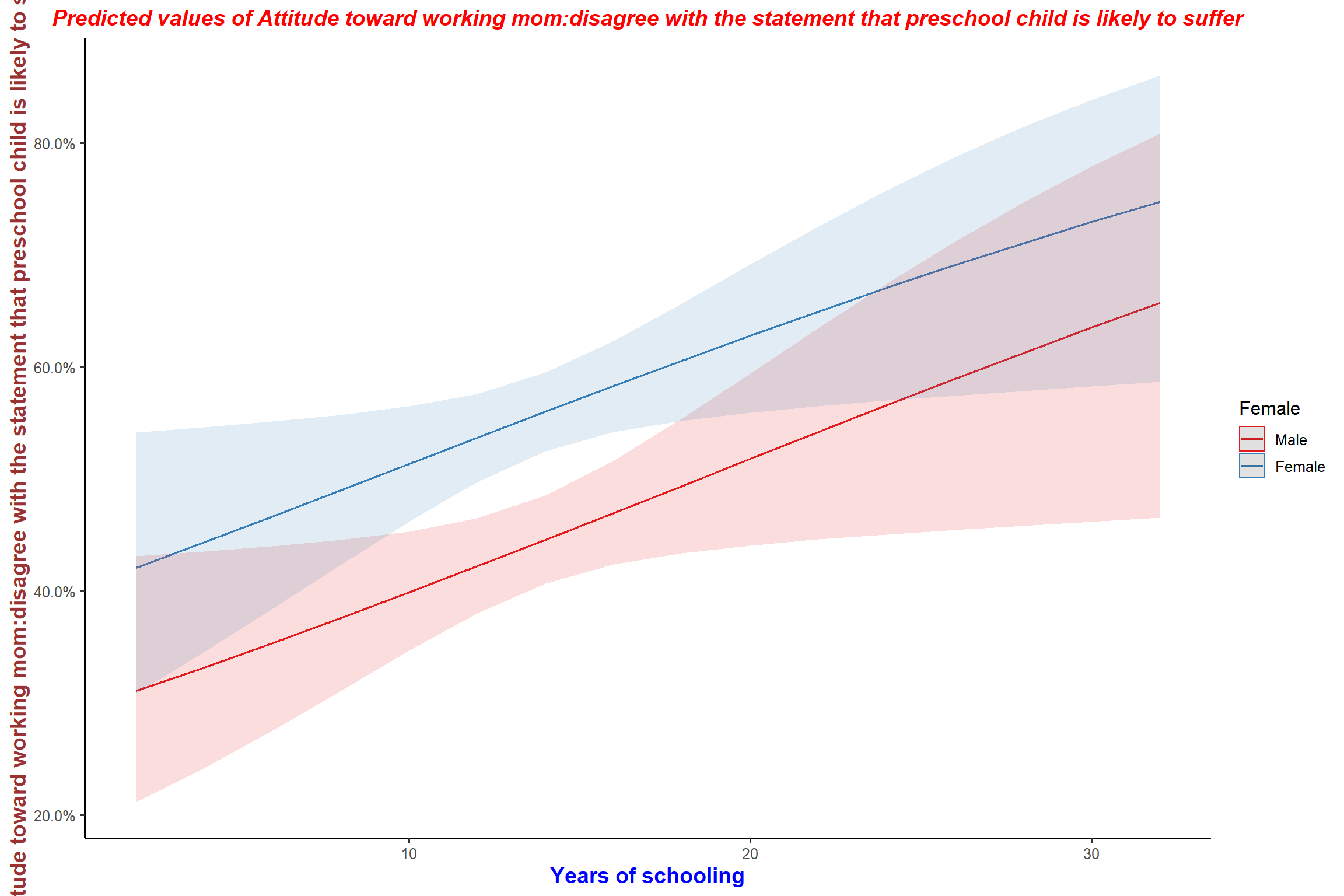
mod4 <- glm(fepresch_d ~ age + educyrs * female, data = mydata, family = "binomial")
summary(mod4)
##
## Call:
## glm(formula = fepresch_d ~ age + educyrs * female, family = "binomial",
##     data = mydata)
##
## Deviance Residuals:
##    Min      1Q  Median      3Q     Max
##  -1.66   -1.14    0.82    1.12    1.67
##
## Coefficients:
##                 Estimate Std. Error z value   Pr(>|z|)
## (Intercept)      0.02600    0.38648    0.07      0.946
## age             -0.01753    0.00357   -4.91 0.00000091 ***
## educyrs          0.04825    0.02155    2.24      0.025 *
## female1          0.47891    0.41105    1.17      0.244
## educyrs:female1 -0.00140    0.02889   -0.05      0.961
## ---
## Signif. codes:  0 '***' 0.001 '**' 0.01 '*' 0.05 '.' 0.1 ' ' 1
##
## (Dispersion parameter for binomial family taken to be 1)
##
##     Null deviance: 2001.6  on 1443  degrees of freedom
## Residual deviance: 1926.7  on 1439  degrees of freedom
##   (168 observations deleted due to missingness)
## AIC: 1937
##
## Number of Fisher Scoring iterations: 4
# Odds ratio plot
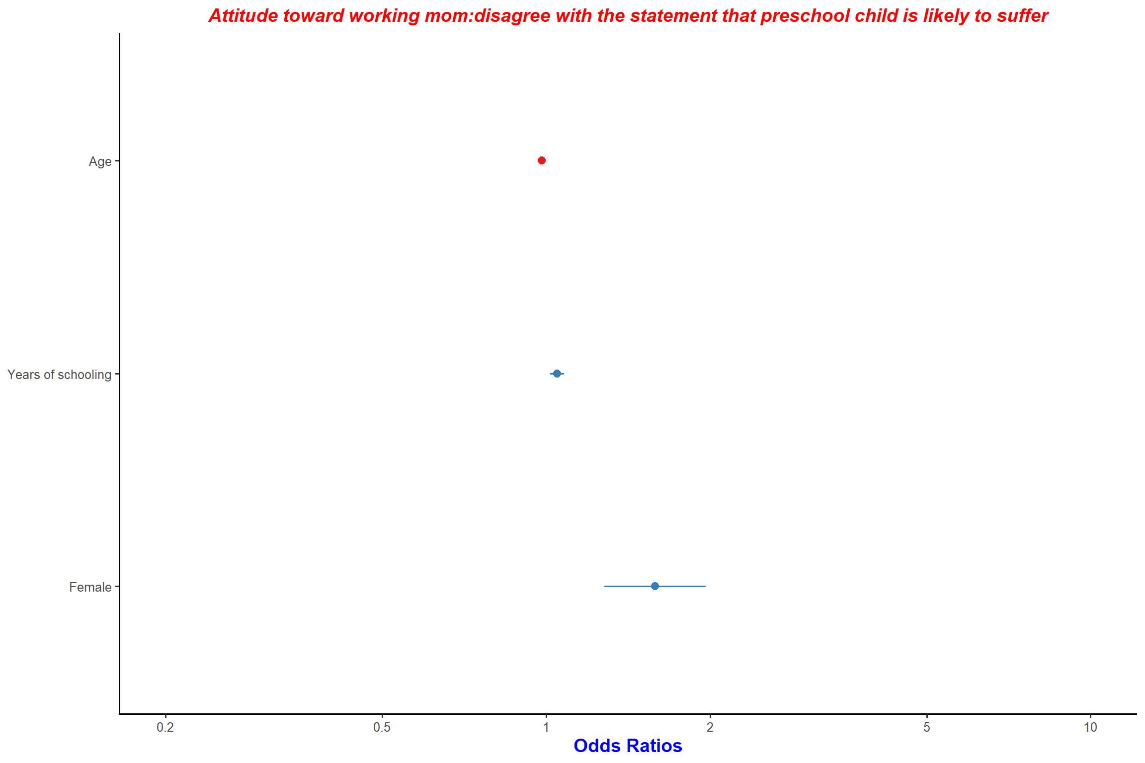
plot_model(mod3, type = "est", wrap.title = 100) + my_theme
# Plot predicted values
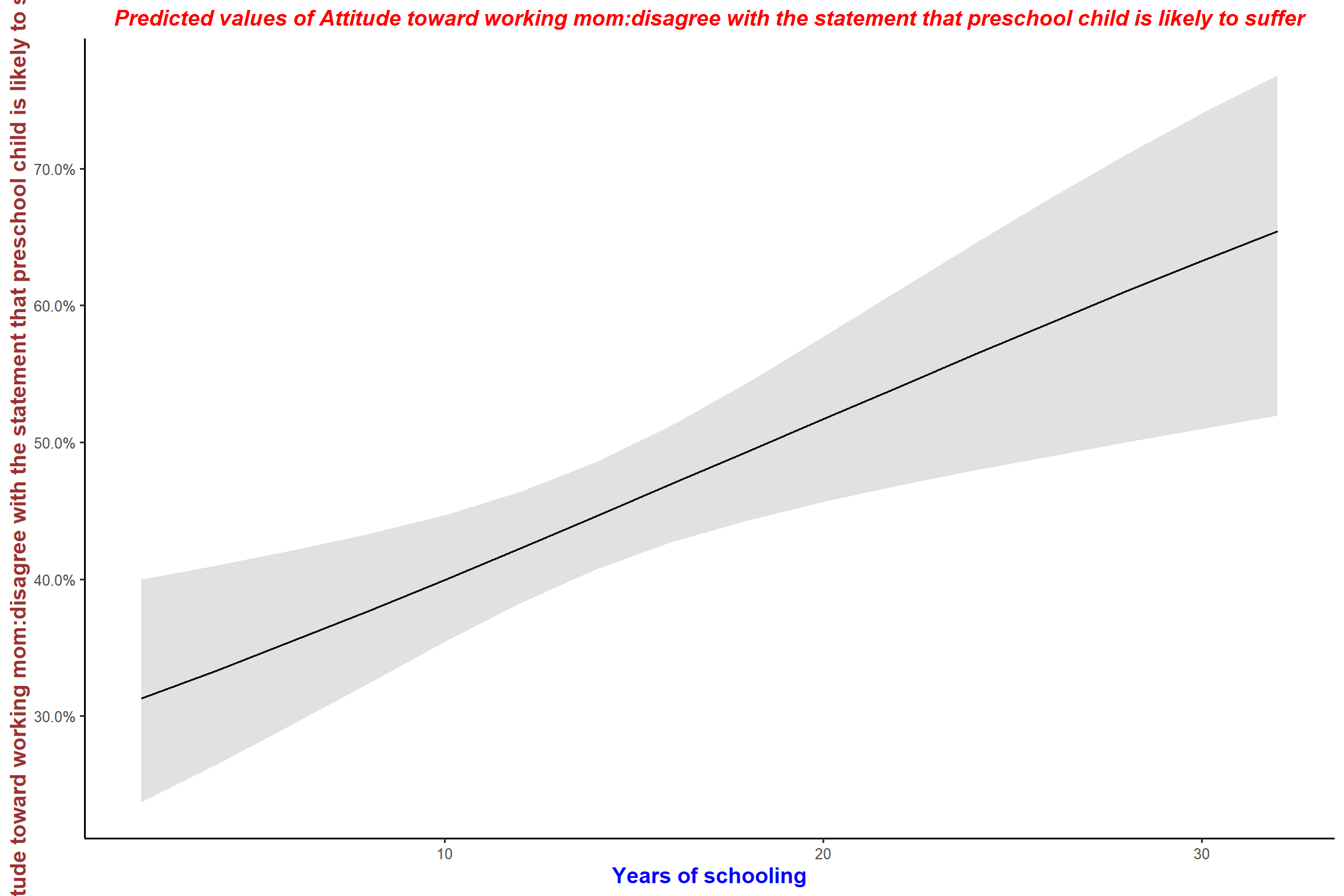
plot_model(mod3, type = "pred", terms = "educyrs") + my_theme
plot_model(mod3, type = "pred", terms = "age") + my_theme
plot_model(mod3, type = "pred", terms = "female") + my_theme
# Plot interaction effect
plot_model(mod4, type = "int") + my_theme
Last updated on 21 October, 2019 by Dr Nicholas Harrigan (nicholas.harrigan@mq.edu.au)